NLP 100 Knocks Summary
Notes on insights gained from the NLP 100 Knocks exercises.
Preparation (Chapter 1)
n-gram
Splitting a string into segments of "n" characters (or words).
Character-level split, N=2 bigram
'今日', '日は', 'はい', 'いい', 'い天', '天気', '気で', 'です', 'すね', 'ね。'
Character-level split, N=3 trigram
'今日は', '日はい', 'はいい', 'いい天', 'い天気', '天気で', '気です', 'ですね', 'すね。'
N-grams are used in NLP preprocessing and also in the BLEU score, an evaluation metric for machine translation. In Japanese, compared to morphological analysis which splits sentences into individual words, n-grams have the advantage of handling unknown words. They eliminate the effort of building a dictionary and can capture co-occurrence patterns, so they are still quietly used widely today. (However, they also introduce a lot of noise.)
UNIX Commands (Chapter 2)
Simple file operations are much more convenient and handy than using Python.
wc -l {file} # Output the number of lines. word count (wc), l probably stands for line.
# 1100, etc.
sed 's/\t/ /g' {file}  # Rewrite file contents. Stream EDitor (sed).
# Replaces tabs with spaces in the file
Regular Expressions (Chapter 3: regex)
json
Python's json library was used to load the dataset.
import json
dic = json.loads('{"bar":["baz", null, 1.0, 2]}')
print(type(dic))
print(dic)
# out
#<class 'dict'>
#{'bar': ['baz', None, 1.0, 2]}
The "s" in loads and dumps does not indicate third-person singular -- it stands for "string."
jsonlines
Saving in jsonl format, where each element is separated by a newline, makes the data easier to read.
import pandas as pd

df.to_json("filename.jsonl",orient='records', lines=True))
# {"col1":1,"col2":"a"}
# {"col1":2,"col2":"x"}
# {"col1":3,"col2":"\u3042"}
regex
A method for specifying string patterns using symbols. I found that the following approach improves readability.
import re
pattern = re.compile(r"""
        \[\[        # [[
        ([^|]+\|)*  # article name|  may be absent or repeated
        ([^]]+)     # display text: replace the matched portion with this
        \]\]        # ]]
    """, re.VERBOSE)
Capture Groups
You can extract strings matched by ( ) in order using \1, \2, ... \n.
text = "2016-05-08"
pattern = re.compile(r'(\d+)-(\d+)-(\d+)')
pattern.sub(r'\1年\2月\3��日', text)
# => 2016年05月08日
Morphological Analysis (Chapter 4: MeCab)
Unlike English, Japanese NLP faces the challenge that word boundaries are not clearly defined. In English, you can simply split by spaces: "Hello World." -> ["hello", "world"]. MeCab can split Japanese sentences into individual words.
import MeCab
wakati = MeCab.Tagger("-Owakati")
words = wakati.parse("ここではきものを脱いでください")
print(words)
#ここ で は きもの を 脱い で ください
There is also a faster alternative called ginza. Explanation of ginza and spaCy
Dependency Parsing (Chapter 5: CaboCha)
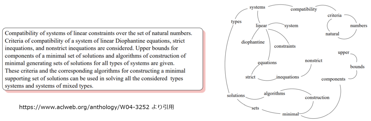
This analyzes dependency relationships such as modifier relations between words. It is used, for example, when solving keyword extraction as a graph problem (the more edges converge on a node, the more important it is). ginza can also be used here.
  Number  Phrase          Head
------  ----------  --------
     0  吾輩は             5
     1  ここで             2
     2  始めて             3
     3  人間という         4
     4  ものを             5
     5  見た。            -1
Machine Learning (Chapter 6: PyTorch)
The task was to classify English news titles into their categories (4 types: business, science, etc.) using logistic regression. Bag of Words (word counts) was used as the feature representation.
Bag of Words
Using the number of unique word types as the dimensionality, a vector is created by counting the occurrences of each word in a given document. Word order is not reflected. Despite its simplicity, it can achieve reasonable accuracy in tasks like document category classification.
Dataset
A class that loads problem-answer (label) pairs. It includes preprocessing. Created for train, validation, and test splits.
DataLoader
A class that determines how to retrieve data from a Dataset. It creates batches (groups of multiple data samples bundled together for simultaneous training).
- In the DataLoader, words are represented as IDs, not vectors. This is because holding word data in vector form would consume a large amount of memory. The model's embedding layer converts IDs to vectors.
nn.Module() and forward
This module, which handles the network layers, follows the basic format shown below.
import torch.nn as nn
import torch.nn.functional as F

class Model(nn.Module):  # Note: nn.Module, not nn.Module()
    def __init__(self,arg*):     # Called the constructor. Executed once when Model() is declared. arg* are the "arguments" of Model()
        super().__init__()   # Inherit the parent class constructor so it is not discarded.
        # Describe network layers here: net1, 2, 3, etc. Below is an example with 2 convolution layers.
        self.conv1 = nn.Conv2d(1, 20, 5)  # In addition to self.conv1 and conv2 defined above,
        self.conv2 = nn.Conv2d(20, 20, 5) # variables declared in nn.Module's constructor (e.g., self.training) can also be used.

    def forward(self, x):  # Executed via nn.Module's __call__ function when Model()(x) is called.
        x = F.relu(self.conv1(x))
        return F.relu(self.conv2(x))  # The return of forward is the return of Model()()
Loss Function
Computes the discrepancy between the model's prediction and the actual answer.
Optimizer
Updates the weights. The model's weights are passed via model.parameters(). Weights are stored in attributes like Model.conv1.weight.
Logistic Regression
The perceptron optimizes (i.e., trains) the weights a and bias b in y=ax+b using a loss function (hinge loss) and an optimization algorithm. A step function that outputs binary values ([0,1] or [-1,1]) is used as the activation function. Hinge loss: (true value) - (predicted value)^2
In contrast, logistic regression uses a sigmoid function for activation, cross-entropy as the loss function, and includes a regularization term to prevent overfitting.
Both the perceptron and logistic regression are algorithms that separate linearly separable targets. (They classify by drawing a line and determining which side a sample falls on.)
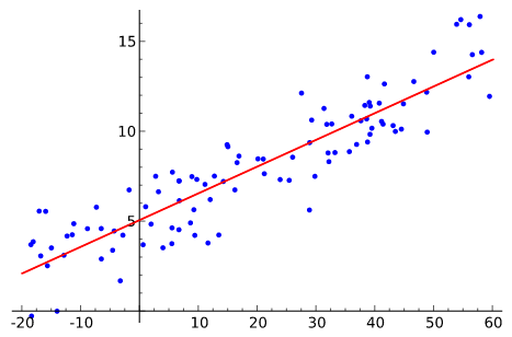
Figure from Wikipedia
Performance Evaluation
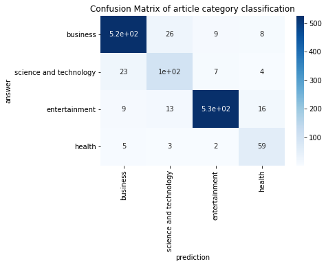
Confusion Matrix
A plot of the actual counts (n) for the model's predictions (x) versus the true answers (y). The more the numbers concentrate along the diagonal from top-left to bottom-right, the better the accuracy.
Recall (accuracy among actual positives) and Precision (accuracy when predicted as positive)
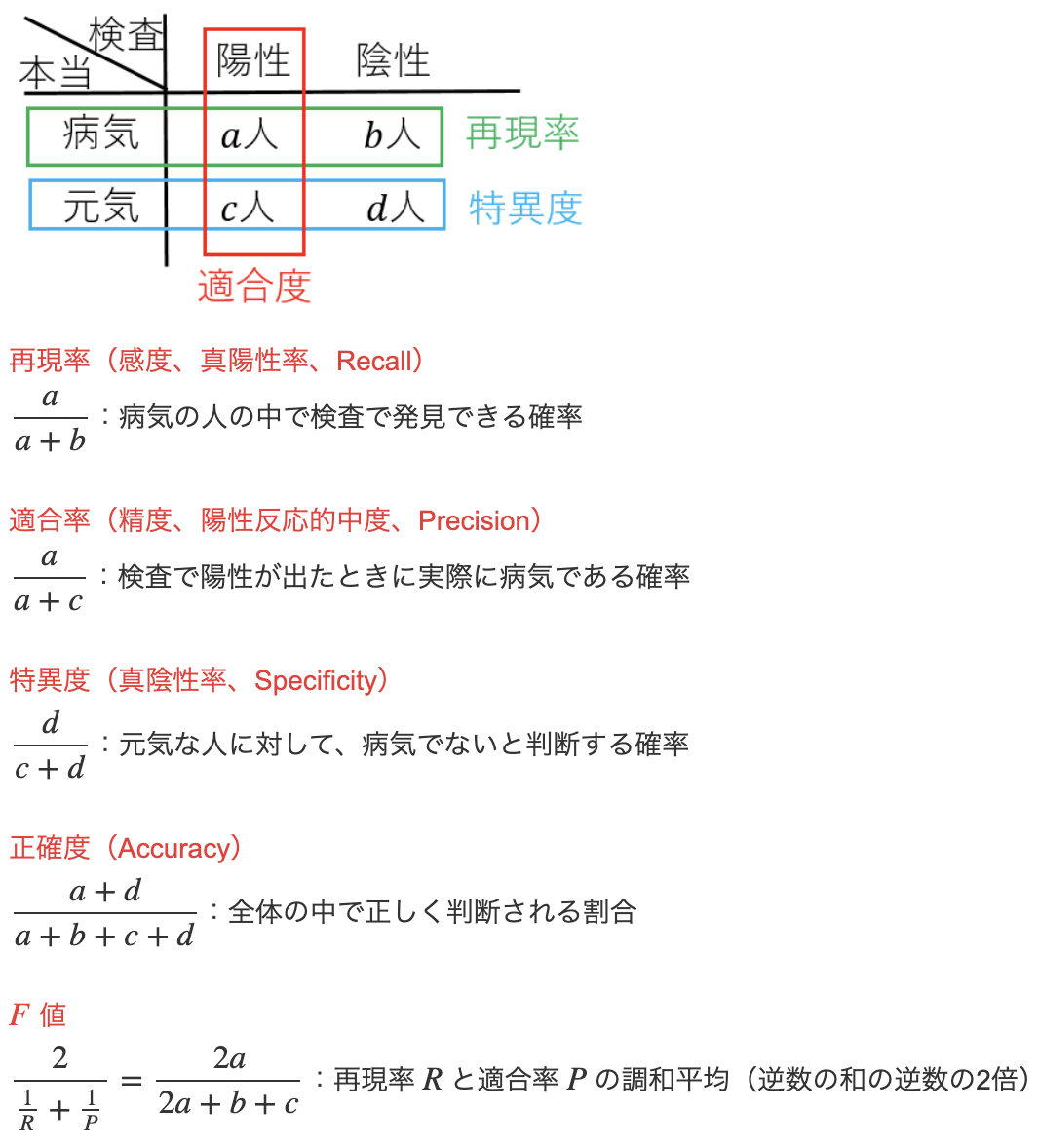 Source: https://mathwords.net/kensa
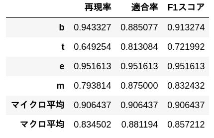
Micro average: An average that ignores label classes (does not distinguish between b, t, e, m below)
Macro average: An average computed as the sum of per-class probabilities divided by the number of classes
Given a task of classifying sentences into b, t, e, and m, the result would look like the following:
Word Vectors (Chapter 7)
A pre-trained model that outputs word vectors was used.
from gensim.models import KeyedVectors
model = KeyedVectors.load_word2vec_format('GoogleNews-vectors-negative300.bin.gz', binary=True)
model["United_States"]  # model[word]
word2vec includes algorithms such as CBOW and skip-gram. They work by masking a word in a sentence and having the machine learning model predict the hidden word. The weights produced when a word is fed into the model are then used as the word vector. Just as RGB values indicate color proximity (e.g., turquoise=(0,183,206) and cyan=(0,174,239)), word vectors enable measuring semantic similarity between words (e.g., using cosine similarity).
Semantic Analogy and Syntactic Analogy
Semantic analogy: Inference based on the semantic relationships of words. man + queen = king
Syntactic analogy: Inference based on the grammatical relationships of words. "eat -> ate" implies "cook -> cooked"
Neural Networks (Chapter 8)
Neural network: A multi-layer version of the perceptron with modified activation functions. (Step function -> sigmoid function, ReLU function, etc.)
In this exercise, the feature representation treated each sentence as the average of its word vectors. There are also methods to directly vectorize sentences (e.g., BERT model, SCDV(Sparse Composite Document Vector), etc.)
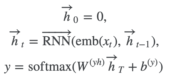
RNN (LSTM) (Chapter 9)
RNNs can take into account the order of words in a sentence. However, since the hidden state vector h used in RNNs is heavily influenced by the immediately preceding word vector, Self-Attention, which can reference word vectors in the sentence with arbitrary weights, is generally preferred.
https://qiita.com/t_Signull/items/21b82be280b46f467d1b
 However,
  Quoted from NLP100Knock
Machine Translation (Chapter 10: fairseq)
(fairseq-train requires PyTorch >= 1.4 and a GPU)
This stands for Facebook AI Research Sequence-to-Sequence Toolkit. It allows you to train machine translation models such as LSTM, Transformer, and BERT_base from the command line.
fairseq-preprocess # Creates dictionaries and binarizes data.
faiseq-train # Trains using GPU. Can also save TensorBoard logs. Is there a CPU argument?
from fairseq.models.transformer import TransformerModel
model = TransformerModel.from_pretrained('path/to/checkpoint_dir', checkpoint_file = 'model.pt')
model.translate("Hello world.")
# 世界の皆さんこんにちは。(For a Japanese-to-English machine translation model)
Transformer
When we translate from Japanese to English, we translate based on specific words (e.g., cat -> neko).
The hidden state vector in RNNs is heavily influenced by the immediately preceding word, but a vector strongly influenced by a specific (not necessarily adjacent) word is more desirable.
Additionally, RNNs cannot fully utilize GPUs.
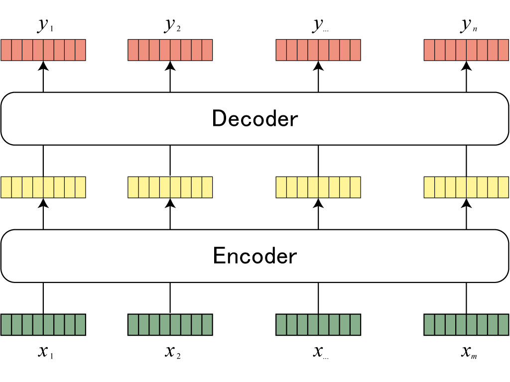
The Transformer is a model that uses a technique called Attention to address these problems.
Input sentence word vectors (green), Attention (yellow), translated words (orange)
 This explanation of Attention was easy to understand:
https://qiita.com/Kosuke-Szk/items/d49e2127bf95a1a8e19f
This explanation of Attention was easy to understand:
https://qiita.com/Kosuke-Szk/items/d49e2127bf95a1a8e19f
BLEU Score
It is based on the premise that the more a machine-generated sentence resembles a human translation, the more likely it is to be correct. The score measures how closely the n-grams of the translated sentence match those of the reference sentence. Typically, 4-gram is commonly used. A score closer to 100 indicates better performance; Transformers reportedly achieve around 20. https://to-in.com/blog/102282
fairseq-score --sys translated.spacy --ref test.spacy.en
#Namespace(ignore_case=False, order=4, ref='test.spacy.en', sacrebleu=False, sentence_bleu=False, sys='98_2.out.spacy')
#BLEU4 = 11.07, 36.2/14.0/7.2/4.1 (BP=1.000, ratio=1.129, syslen=31201, reflen=27625)
BLEU scores will penalize synonyms as incorrect, but BERTScore compares sentence vectors and is said to handle this issue.
Beam Search
A method that extends breadth-first search by further exploring up to a specified beam width. In machine translation, by only considering sentences starting with the highest-probability words (up to the beam width), computational cost can be reduced.
N=5 # Beam width
fairseq-interactive --path checkpoint.pt --beam $N data
Subword
A method of splitting infrequent words into units of a few characters. Compared to traditional word-level preprocessing, character-level splitting reduces vocabulary size and thus computational cost, while also eliminating unknown words. https://qiita.com/NLPingu/items/78f11ec4c3b777f56f11
fasttext is reportedly word2vec with subword techniques incorporated.
subword-nmt learn-bpe -s 3000 < wakati_wagahai.txt > codes.txt
subword-nmt apply-bpe -c codes.txt < wakati_wagahai.txt > subword_wagahai.txt
# The rain@@ y season began in the southern area of Kyushu around May@@ .@@ 31 (F@@ ri@@ ) as norm@@ al.
# rain@@y indicates that it was originally the single word "rainy".
While subword refers to word -> character segments, SentencePiece refers to sentence -> character segments. It is said that recent state-of-the-art machine learning models use this approach.
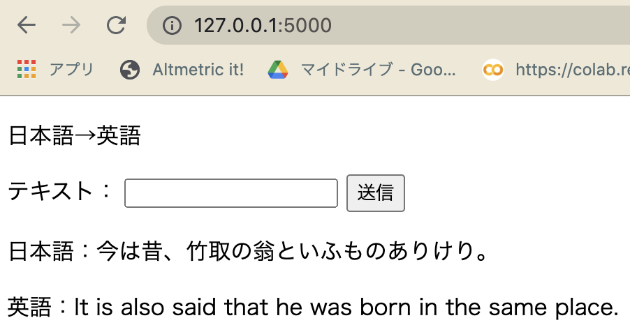
Machine Translation Results
A Transformer model (.pt) trained on translating classical Japanese to English using fairseq was deployed using flask.
The accuracy is mediocre...