[Never Again] Understanding RNN and LSTM with NumPy Implementation
This article covers methods for learning sequential data using neural networks. Learning sequential data has various applications such as word prediction and weather forecasting.
The explanation follows this flow:
- How to represent categorical variables in neural networks
- How to implement RNN
- How to implement LSTM
- How to implement LSTM using PyTorch
Representing Time Series Data
To input time series data into a neural network, the data needs to be represented in a form that the neural network can accept. Here, we will use one-hot encoding.
One-hot Encoding for Words
We convert words into one-hot vectors. However, when the vocabulary becomes enormous, the one-hot vector size also becomes enormous, so we apply some techniques.
We keep the top k most frequently used words and convert all other words to UNK, then transform them into one-hot vectors.
Generating the Dataset
Consider generating a dataset like:
a b a EOS,
a a b b a a EOS,
a a a a a b b b b b a a a a a EOS
EOS stands for end of a sequence.
import numpy as np

np.random.seed(42)#Fix random seed

def generate_dataset(num_sequences=2**8):
    """
    Function to generate dataset
    num_sequences: number of sequences
    return: list of sequential data
    """
    samples = []

    for _ in range(num_sequences):
        num_tokens = np.random.randint(1, 6)#Generate one number from 1 to 6
        sample = ['a'] * num_tokens + ['b'] * num_tokens + ['a'] * num_tokens + ['EOS']
        samples.append(sample)

    return samples

sequences = generate_dataset()
Examining Words and Their Frequencies in Sequential Data
To perform one-hot encoding, we create a dictionary that stores the words in the sequential data and their frequencies.
By using defaultdict, you can initialize dictionary values to arbitrary values.
from collections import defaultdict

def sequences_to_dicts(sequences):
    """
    Create a dictionary storing words and their frequencies
    """
    flatten = lambda l: [item for sublist in l for item in sublist]#Concatenate all lists

    all_words = flatten(sequences)

    word_count = defaultdict(int)#Initialize dictionary
    for word in flatten(sequences):
        #Count frequencies
        word_count[word] += 1

    word_count = sorted(list(word_count.items()), key=lambda l: -l[1])#Sort word_count keys and values in descending order by value

    unique_words = [item[0] for item in word_count]#Extract words

    unique_words.append('UNK')#Add UNK

    num_sequences, vocab_size = len(sequences), len(unique_words)

    word_to_idx = defaultdict(lambda: vocab_size-1)#Set default value
    idx_to_word = defaultdict(lambda: 'UNK')


    for idx, word in enumerate(unique_words):
        #Get index and element with enumerate
        #Store in dictionary
        word_to_idx[word] = idx
        idx_to_word[idx] = word

    return word_to_idx, idx_to_word, num_sequences, vocab_size

word_to_idx, idx_to_word, num_sequences, vocab_size = sequences_to_dicts(sequences)
Splitting the Dataset
We split the sequential data into training, validation, and test sets. The split is 80%, 10%, and 10% respectively. Slicing is used to split the sequential data.
Using slicing, l[start:goal] extracts values from l[start] to l[goal-1]. start and goal form a half-open interval, so l[goal] is not included.
start and goal can be omitted.
l[:goal] extracts from l[0] to l[goal-1],
l[start:] extracts from l[start] to l[l.size()-1] (the end).
l[:] extracts everything.
l[-n:] extracts the last n elements.
l[:-n] extracts from l[0] but excludes the last n elements.
We define the dataset using PyTorch.
from torch.utils import data

class Dataset(data.Dataset):
    def __init__(self, inputs, targets):
        self.intputs = inputs
        self.targets = targets

    def __len__(self):
        return len(self.targets)

    def __getitem__(self, index):
        X = self.inputs[index]
        y = self.targets[index]

        return X, y

def create_datasets(sequences, dataset_class, p_train=0.8, p_val=0.1, p_test=0.1):
    #Define split sizes
    num_train = int(len(sequences)*p_train)
    num_val = int(len(sequences)*p_val)
    num_test = int(len(sequences)*p_test)

    #Split the sequential data
    #Using slicing
    sequences_train = sequences[:num_train]
    sequences_val = sequences[num_train:num_train+num_val]
    sequences_test = sequences[-num_test:]

    def get_inputs_targets_from_sequences(sequences):
        inputs, targets = [], []

        #L-1 after removing EOS from a sequence of length L
        # targets are shifted right by 1 as ground truth for inputs
        for sequence in sequences:
            inputs.append(sequence[:-1])
            targets.append(sequence[1:])

        return inputs, targets

    #Create inputs and targets
    inputs_train, targets_train = get_inputs_targets_from_sequences(sequences_train)
    inputs_val, targets_val = get_inputs_targets_from_sequences(sequences_val)
    inputs_test, targets_test = get_inputs_targets_from_sequences(sequences_test)

    #Create datasets using the previously defined class
    training_set = dataset_class(inputs_train, targets_train)
    validation_set = dataset_class(inputs_val, targets_val)
    test_set = dataset_class(inputs_test, targets_test)

    return training_set, validation_set, test_set

training_set, validation_set, test_set = create_datasets(sequences, Dataset)
One-hot Vector Encoding
We convert words appearing in the sequential data into one-hot vectors based on their frequency.
def one_hot_encode(idx, vocab_size):
    """
    Convert to one-hot vector.
    """
    one_hot = np.zeros(vocab_size)#If vocab_size = 4, then [0, 0, 0, 0]
    one_hot[idx] = 1.0#If idx = 1, then [0, 1, 0, 0]
    return one_hot

def one_hot_encode_sequence(sequence, vocab_size):
    """
    return 3-D numpy array (num_words, vocab_size, 1)
    """
    encoding = np.array([one_hot_encode(word_to_idx[word], vocab_size) for word in sequence])

    #reshape
    encoding = encoding.reshape(encoding.shape[0], encoding.shape[1], 1)

    return encoding
Introduction to RNN
Recurrent neural networks (RNNs) excel at analyzing sequential data. RNNs can use computation results from previous states in the current state. The network overview diagram is shown below.
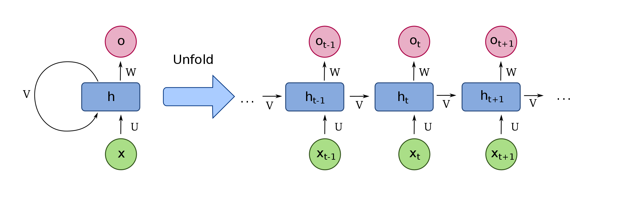
- x is the input sequential data
- U is the weight matrix for the input
- V is the weight matrix for the memory
- W is the weight matrix for the hidden state used to compute the output
- h is the hidden state (memory) at each time step
- o is the output
RNN Implementation
We implement the RNN using NumPy, in the order of forward pass, backward pass, optimization, and training loop.
RNN Initialization
We define a function to initialize the network.
hidden_size = 50#Dimension of the hidden layer (memory)
vocab_size = len(word_to_idx)

def init_orthogonal(param):
    """
    Initialize parameters with orthogonal initialization
    """

    if param.ndim < 2:
        raise ValueError("Only parameters with 2 or more dimensions are supported.")

    rows, cols = param.shape

    new_param = np.random.randn(rows, cols)

    if rows < cols:
        new_param = new_param.T

    q, r = np.linalg.qr(new_param)

    d = np.diag(r, 0)
    ph = np.sign(d)
    q *= ph

    if rows < cols:
        q = q.T

    new_param = q

    return new_param

def init_rnn(hidden_size, vocab_size):
    """
    Initialize RNN
    """
    U = np.zeros((hidden_size, vocab_size))
    V = np.zeros((hidden_size, hidden_size))
    W = np.zeros((vocab_size, hidden_size))
    b_hidden = np.zeros((hidden_size, 1))
    b_out = np.zeros((vocab_size, 1))

    U = init_orthogonal(U)
    V = init_orthogonal(V)
    W = init_orthogonal(W)

    return U, V, W, b_hidden, b_out
Implementing Activation Functions
We implemented sigmoid, tanh, and softmax. A small epsilon is added to the input x to prevent overflow. Derivatives are also computed for the backward pass.
def sigmoid(x, derivative=False):
    x_safe = x + 1e-12#Add small epsilon
    f = 1/(1 + np.exp(-x_safe))

    if derivative:
        return f * (1 -f)#Return derivative
    else:
        return f

def tanh(x, derivative=False):
    x_safe = x + 1e-12
    f = (np.exp(x_safe) - np.exp(-x_safe))/(np.exp(x_safe)+np.exp(-x_safe))

    if derivative:
        return 1-f**2
    else:
        return f

def softmax(x, derivative=False):
    x_safe = x + 1e-12
    f = np.exp(x_safe)/np.sum(np.exp(x_safe))

    if derivative:
        pass
    else:
        return f
Implementing the Forward Pass
- h = tanh(Ux + Vh + b_hidden)
- o = softmax(Wh + b_out) The RNN forward pass is expressed by the equations above, so the implementation is as follows:
def forward_pass(inputs, hidden_state, params):
    U, V, W, b_hidden, b_out = params

    outputs, hidden_states = [], []

    for t in range(len(inputs)):
        hidden_state = tanh(np.dot(U, inputs[t]) + np.dot(V, hidden_state) + b_hidden)

        out = softmax(np.dot(W, hidden_state) + b_out)
        outputs.append(out)
        hidden_states.append(hidden_state.copy())

    return outputs, hidden_states
Implementing the Backward Pass
Computing loss gradients in the forward pass is time-consuming, so we implement a backward pass that computes gradients using backpropagation.
We create a function to clip gradients as a countermeasure against exploding gradients. When the gradient magnitude exceeds the upper limit, it is normalized by the upper limit.
def clip_gradient_norm(grads, max_norm=0.25):
    """
    As a countermeasure against exploding gradients,
    transform gradients to
    g = (max_norm/|g|)*g
    """
    max_norm = float(max_norm)
    total_norm = 0

    for grad in grads:
        grad_norm = np.sum(np.power(grad, 2))
        total_norm += grad_norm

    total_norm = np.sqrt(total_norm)

    clip_coef = max_norm / (total_norm + 1e-6)

    if clip_coef < 1:
        for grad in grads:
            grad *= clip_coef

    return grads
We create a function to compute the backward pass. It calculates the loss and then computes the gradients of the loss differentiated with respect to each parameter using backpropagation.
def backward_pass(inputs, outputs, hidden_states, targets, params):
    U, V, W, b_hidden, b_out = params

    d_U, d_V, d_W = np.zeros_like(U), np.zeros_like(V), np.zeros_like(W)
    d_b_hidden, d_b_out = np.zeros_like(b_hidden), np.zeros_like(b_out)

    d_h_next = np.zeros_like(hidden_states[0])
    loss = 0

    for t in reversed(range(len(outputs))):
        #Compute cross entropy loss
        loss += -np.mean(np.log(outputs[t]+1e-12)*targets[t])

        #backpropagate into output
        d_o = outputs[t].copy()
        d_o[np.argmax(targets[t])] -= -1

        #backpropagate into W
        d_W += np.dot(d_o, hidden_states[t].T)
        d_b_out += d_o

        #backpropagate into h
        d_h = np.dot(W.T, d_o) + d_h_next

        #backpropagate through non-linearity
        d_f = tanh(hidden_states[t], derivative=True) * d_h
        d_b_hidden += d_f

        #backpropagate into U
        d_U += np.dot(d_f, inputs[t].T)

        #backpropagate into V
        d_V += np.dot(d_f, hidden_states[t-1].T)
        d_h_next = np.dot(V.T, d_f)

    grads = d_U, d_V, d_W, d_b_hidden, d_b_out

    grads = clip_gradient_norm(grads)

    return loss, grads
optimization
We update the RNN parameters using gradient descent. This time we use Stochastic Gradient Descent (SGD).
def update_paramaters(params, grads, lr=1e-3):
    for param, gras in zip(params, grads):
        #Get elements from multiple lists using zip
        param -= lr * grad

    return params
Training
We train the implemented RNN. The loss graph was plotted using TensorBoard.
from torch.utils.tensorboard import SummaryWriter

writer = SummaryWriter(log_dir="./logs")#Create SummaryWriter instance and specify save directory

num_epochs = 1000

#Initialize parameters
params = init_rnn(hidden_size=hidden_size, vocab_size=vocab_size)

hidden_state = np.zeros((hidden_size, 1))

for i in range(num_epochs):

    epoch_training_loss = 0
    epoch_validation_loss = 0

    #Validation loop, iterating over each sentence
    for inputs, targets in validation_set:
        #One-hot vector encoding
        inputs_one_hot = one_hot_encode_sequence(inputs, vocab_size)
        targets_one_hot = one_hot_encode_sequence(targets, vocab_size)

        #Initialize
        hidde_state = np.zeros_like(hidden_state)

        #forward pass
        outputs, hidden_states = forward_pass(inputs_one_hot, hidden_state, params)

        #backward pass: only compute loss since this is validation
        loss, _ = backward_pass(inputs_one_hot, outputs, hidden_states, targets_one_hot, params)

        epoch_validation_loss += loss

    #Training loop, iterating over each sentence
    for inputs, targets in training_set:
        #One-hot vector encoding
        inputs_one_hot = one_hot_encode_sequence(inputs, vocab_size)
        targets_one_hot = one_hot_encode_sequence(targets, vocab_size)

        #Initialize
        hidde_state = np.zeros_like(hidden_state)

        #forward pass
        outputs, hidden_states = forward_pass(inputs_one_hot, hidden_state, params)

        #backward pass: also compute gradients since this is training
        loss, grads = backward_pass(inputs_one_hot, outputs, hidden_states, targets_one_hot, params)

        if np.isnan(loss):
            raise ValueError('Gradients have vanished')

        #Update network parameters
        params = update_paramaters(params, grads)

        epoch_training_loss += loss

    writer.add_scalars("Loss", {"val":epoch_validation_loss/len(validation_set), "train":epoch_training_loss/len(training_set)}, i)

writer.close()
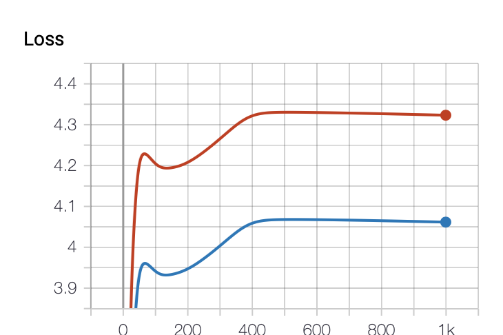
This is the loss graph. It is plotted cleanly. Red represents train, and blue represents val. We can see that the learning is not going very well. This might be due to the small dimension of the hidden layer, the low number of iterations, or inappropriate initial parameter values.
Testing
We test the trained RNN. We generate arbitrary sentences and predict the next word for each.
In Python, list[-1] can be used to get the last element.
def freestyle(params, sentence='', num_generate=10):
    sentence = sentence.split(' ')#Split by spaces
    sentence_one_hot = one_hot_encode_sequence(sentence, vocab_size)

    hidden_state = np.zeros((hidden_size, 1))

    outputs, hidden_states = forward_pass(sentence_one_hot, hidde_state, params)

    output_sentence = sentence

    word = idx_to_word[np.argmax(outputs[-1])]
    output_sentence.append(word)

    for i in range(num_generate):

        output = outputs[-1]#Get the last value
        hidden_state = hidden_states[-1]

        output = output.reshape(1, output.shape[0], output.shape[1])

        outputs, hidden_states = forward_pass(output, hidde_state, params)

        word = idx_to_word[np.argmax(outputs)]

        output_sentence.append(word)

        if word == "EOS":
            break

    return output_sentence


test_examples = ['a a b', 'a a a a b', 'a a a a a a b', 'a', 'r n n']
for i, test_example in enumerate(test_examples):
    print(f'Example {i}:', test_example)
    print('Predicted sequence:', freestyle(params, sentence=test_example), end='\n\n')
Since the learning was not successful, we can see from the results that the testing also did not go well. Everything is predicted as Unknown.
Example 0: a a b
Predicted sequence: ['a', 'a', 'b', 'UNK', 'UNK', 'UNK', 'UNK', 'UNK', 'UNK', 'UNK', 'UNK', 'UNK', 'UNK', 'UNK']

Example 1: a a a a b
Predicted sequence: ['a', 'a', 'a', 'a', 'b', 'UNK', 'UNK', 'UNK', 'UNK', 'UNK', 'UNK', 'UNK', 'UNK', 'UNK', 'UNK', 'UNK']

Example 2: a a a a a a b
Predicted sequence: ['a', 'a', 'a', 'a', 'a', 'a', 'b', 'UNK', 'UNK', 'UNK', 'UNK', 'UNK', 'UNK', 'UNK', 'UNK', 'UNK', 'UNK', 'UNK']

Example 3: a
Predicted sequence: ['a', 'UNK', 'UNK', 'UNK', 'UNK', 'UNK', 'UNK', 'UNK', 'UNK', 'UNK', 'UNK', 'UNK']

Example 4: r n n
Predicted sequence: ['r', 'n', 'n', 'UNK', 'UNK', 'UNK', 'UNK', 'UNK', 'UNK', 'UNK', 'UNK', 'UNK', 'UNK', 'UNK']
Introduction to LSTM
RNNs have difficulty learning to relate information as the gap grows larger. Long Short Term Memory (LSTM) was designed to learn such long-term dependencies. LSTM is a variant of RNN and similarly consists of repeating modules.
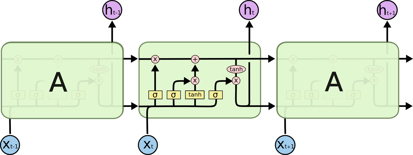
How LSTM Works
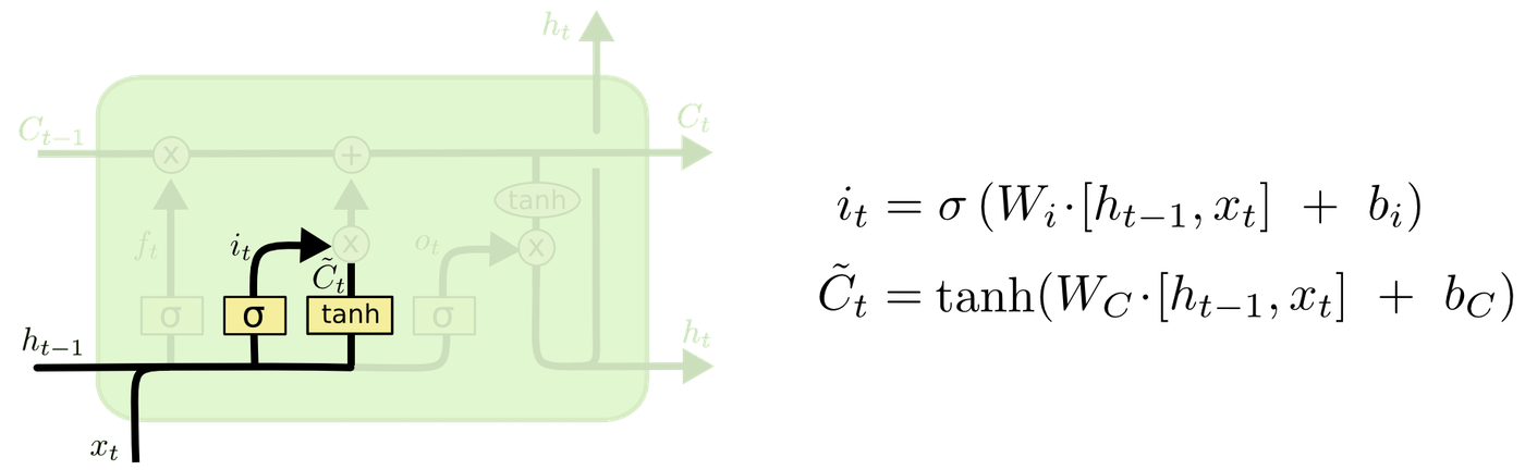
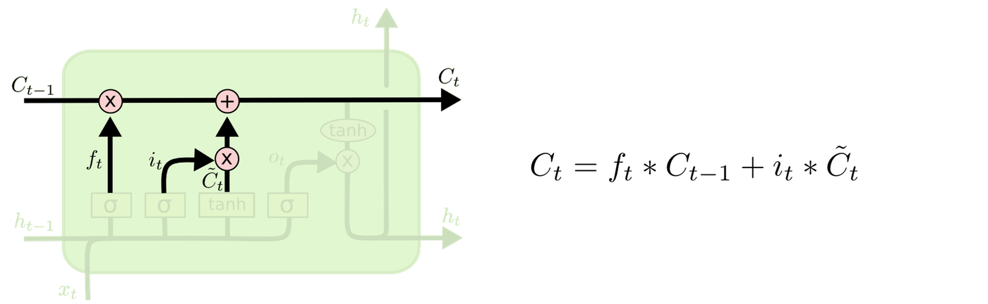
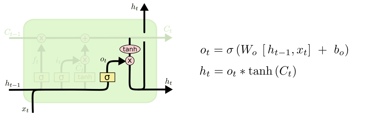
LSTM consists of three components: the forget gate layer, the input gate layer, and the output gate layer. LSTM maintains information through memory units called cells. C represents the cell, x the input, h the output, W the weights, and b the bias.
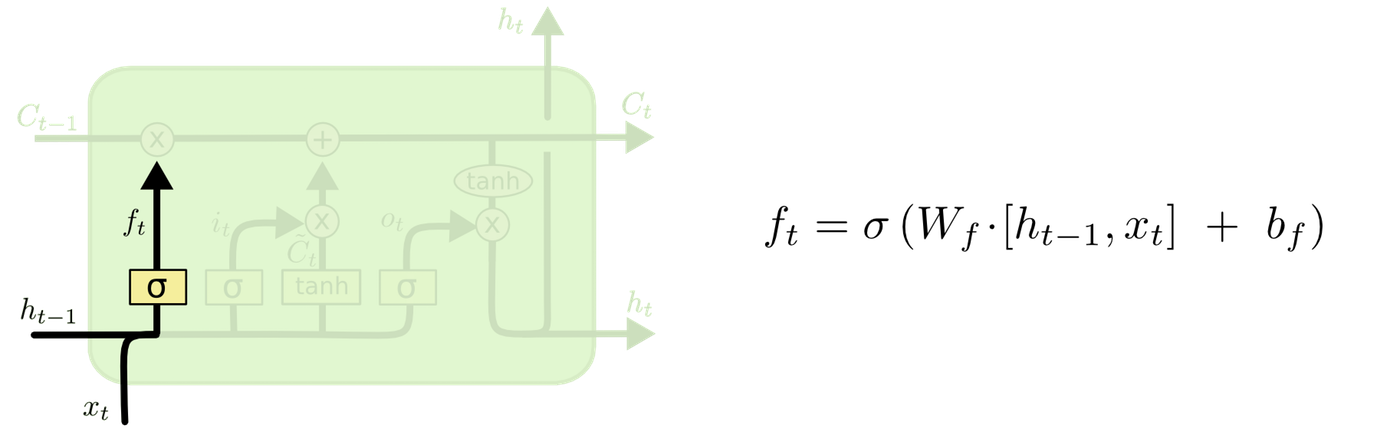
First, the forget gate layer determines which information to discard from the cell state. The current input and the output from the previous step are fed into a sigmoid function. A value between 0 and 1 is output. 0 represents "completely discard" and 1 represents "completely retain."
Next, the input gate layer determines which values to update for the input. The tanh layer creates a vector of new candidate values to be added to the cell state.
The cell is updated. The forgotten cell from the previous step and the values to update are added together.
Finally, the output gate layer determines what to output based on the cell state.
LSTM Implementation
We implement the LSTM using NumPy, in the order of forward pass, backward pass, optimization, and training loop.
LSTM Initialization
We define a function to initialize the network.
z_size = hidden_size + vocab_size

def init_lstm(hidden_size, vocab_size, z_size):
    """
    Initialize LSTM
    """

    W_f = np.random.randn(hidden_size, z_size)

    b_f = np.zeros((hidden_size, 1))

    W_i = np.random.randn(hidden_size, z_size)

    b_i = np.zeros((hidden_size, 1))

    W_g = np.random.randn(hidden_size, z_size)

    b_g = np.zeros((hidden_size, 1))

    W_o = np.random.randn(hidden_size, z_size)
    b_o = np.zeros((hidden_size, 1))

    W_v = np.random.randn(vocab_size, hidden_size)
    b_v = np.zeros((vocab_size, 1))

    W_f = init_orthogonal(W_f)
    W_i = init_orthogonal(W_i)
    W_g = init_orthogonal(W_g)
    W_o = init_orthogonal(W_o)
    W_v = init_orthogonal(W_v)

    return W_f, W_i, W_g, W_o, W_v, b_f, b_i, b_g, b_o, b_v
Implementing the Forward Pass
We implement following the data flow described in the LSTM mechanism section.
def forward(inputs, h_prev, C_prev, p):
    """
    inputs: current input
    h_prev: output from previous step
    C_prev: cell from previous step
    p: LSTM parameters
    return: states of each module and output
    """
    assert h_prev.shape == (hidden_size, 1)
    assert C_prev.shape == (hidden_size, 1)

    W_f, W_i, W_g, W_o, W_v, b_f, b_i, b_g, b_o, b_v = p

    x_s, z_s, f_s, i_s = [], [], [], []
    g_s, C_s, o_s, h_s = [], [], [], []
    v_s, output_s = [], []

    h_s.append(h_prev)
    C_s.append(C_prev)


    for x in inputs:
        #Concatenate input and previous step output
        z = np.row_stack((h_prev, x))
        z_s.append(z)

        #Forget gate
        f = sigmoid(np.dot(W_f, z) + b_f)
        f_s.append(f)

        #Input gate
        i = sigmoid(np.dot(W_i, z) + b_i)
        i_s.append(i)

        #Candidate values to add to cell for current input
        g = tanh(np.dot(W_g, z) + b_g)
        g_s.append(g)

        #Cell update
        C_prev = f * C_prev + i * g
        C_s.append(C_prev)

        #Output gate
        o = sigmoid(np.dot(W_o, z) + b_o)
        o_s.append(o)

        #Produce output
        h_prev = o * tanh(C_prev)
        h_s.append(h_prev)

        v = np.dot(W_v, h_prev) + b_v
        v_s.append(v)

        output = softmax(v)
        output_s.append(output)

    return z_s, f_s, i_s, g_s, C_s, o_s, h_s, v_s, output_s
Implementing the Backward Pass
We compute the loss and then obtain the gradients of the loss differentiated with respect to each parameter using backpropagation.
def backward(z, f, i, g, C, o, h, v, outputs, targets, p = params):
    W_f, W_i, W_g, W_o, W_v, b_f, b_i, b_g, b_o, b_v = p

    #Initialize gradients
    W_f_d = np.zeros_like(W_f)
    b_f_d = np.zeros_like(b_f)

    W_i_d = np.zeros_like(W_i)
    b_i_d = np.zeros_like(b_i)

    W_g_d = np.zeros_like(W_g)
    b_g_d = np.zeros_like(b_g)

    W_o_d = np.zeros_like(W_o)
    b_o_d = np.zeros_like(b_o)

    W_v_d = np.zeros_like(W_v)
    b_v_d = np.zeros_like(b_v)

    #Initialize next cell and hidden state
    dh_next = np.zeros_like(h[0])
    dC_next = np.zeros_like(C[0])

    loss = 0

    for t in reversed(range(len(outputs))):
        #Compute cross entropy loss
        loss += -np.mean(np.log(outputs[t]) * targets[t])
        #Update previous cell
        C_prev = C[t-1]

        dv = np.copy(outputs[t])
        dv[np.argmax(targets[t])] -= 1

        W_v_d += np.dot(dv, h[t].T)
        b_v_d += dv

        dh = np.dot(W_v.T, dv)
        dh += dh_next
        do = dh * tanh(C[t])
        do = sigmoid(o[t], derivative=True)*do

        W_o_d += np.dot(do, z[t].T)
        b_o_d += do

        dC = np.copy(dC_next)
        dC += dh * o[t] * tanh(tanh(C[t]), derivative=True)
        dg = dC * i[t]
        dg = tanh(g[t], derivative=True) * dg

        W_g_d += np.dot(dg, z[t].T)
        b_g_d += dg

        di = dC * g[t]
        di = sigmoid(i[t], True) * di

        W_i_d += np.dot(di, z[t].T)
        b_i_d += di

        df = dC * C_prev
        df = sigmoid(f[t]) * df

        W_f_d += np.dot(df, z[t].T)
        b_f_d += df

        dz = (np.dot(W_f.T, df) + np.dot(W_i.T, di) + np.dot(W_g.T, dg) + np.dot(W_o.T, do))
        dh_prev = dz[:hidden_size, :]
        dC_prev = f[t] * dC

    grads = W_f_d, W_i_d, W_g_d, W_o_d, W_v_d, b_f_d, b_i_d, b_g_d, b_o_d, b_v_d

    grads = clip_gradient_norm(grads)

    return loss, grads
Training
We train the implemented LSTM. The loss graph was plotted using TensorBoard.
writer = SummaryWriter(log_dir="./logs/lstm")#Create SummaryWriter instance and specify save directory

num_epochs = 200#Number of epochs

#Initialize LSTM
z_size = hidden_size + vocab_size
params = init_lstm(hidden_size, vocab_size, z_size)

#Initialize hidden layer
hidden_state = np.zeros((hidden_size, 1))

for i in range(num_epochs):

    epoch_training_loss = 0
    epoch_validation_loss = 0

    #Validation loop, iterating over each sentence
    for inputs, targets in validation_set:
        #One-hot vector encoding
        inputs_one_hot = one_hot_encode_sequence(inputs, vocab_size)
        targets_one_hot = one_hot_encode_sequence(targets, vocab_size)

        #Initialize
        h = np.zeros((hidden_size, 1))
        c = np.zeros((hidden_size, 1))

        #forward pass
        z_s, f_s, i_s, g_s, C_s, o_s, h_s, v_s, outputs = forward(inputs_one_hot, h, c, params)

        #backward pass: only compute loss since this is validation
        loss, _ = backward(z_s, f_s, i_s, g_s, C_s, o_s, h_s, v_s, outputs, targets_one_hot, params)

        epoch_validation_loss += loss

    #Training loop, iterating over each sentence
    for inputs, targets in training_set:
        #One-hot vector encoding
        inputs_one_hot = one_hot_encode_sequence(inputs, vocab_size)
        targets_one_hot = one_hot_encode_sequence(targets, vocab_size)

        #Initialize
        h = np.zeros((hidden_size, 1))
        c = np.zeros((hidden_size, 1))

        #forward pass
        z_s, f_s, i_s, g_s, C_s, o_s, h_s, v_s, outputs = forward(inputs_one_hot, h, c, params)

        #backward pass: compute both loss and gradients since this is training
        loss, grads = backward(z_s, f_s, i_s, g_s, C_s, o_s, h_s, v_s, outputs, targets_one_hot, params)

        #Update LSTM parameters
        params = update_paramaters(params, grads, lr=1e-1)
        epoch_training_loss += loss

    writer.add_scalars("LSTM Loss", {"val":epoch_validation_loss/len(validation_set), "train":epoch_training_loss/len(training_set)}, i)

writer.close()
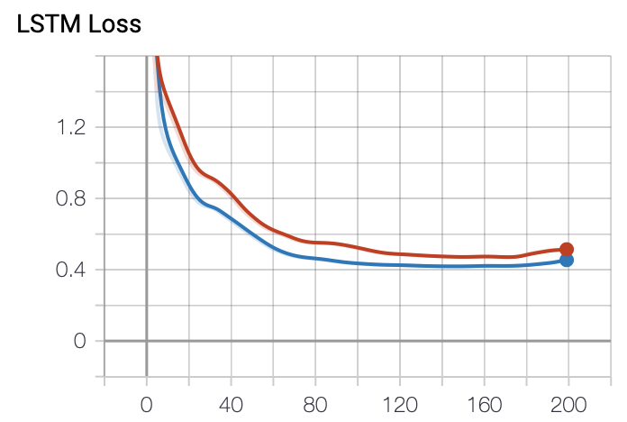
This is the loss graph. It is plotted cleanly. Red represents train, and blue represents val. Compared to the RNN, the loss decreases steadily as training progresses, showing more stable learning.
LSTM Implementation with PyTorch
We implement LSTM using a framework.
Defining the LSTM
First, we define the LSTM network.
import torch
import torch.nn as nn
import torch.nn.functional as F

class MyLSTM(nn.Module):
    def __init__(self):
        super(MyLSTM, self).__init__()
        self.lstm = nn.LSTM(input_size=vocab_size, hidden_size=50, num_layers=1, bidirectional=False)
        self.l_out = nn.Linear(in_features=50, out_features=vocab_size, bias=False)

    def forward(self, x):
        x, (h, c) = self.lstm(x)

        x = x.view(-1, self.lstm.hidden_size)

        x = self.l_out(x)

        return x
Training
We write the training loop. Cross entropy loss is used as the loss function, and SGD is used as the optimizer. This is the same as when using numpy.
In PyTorch, when using cross entropy loss, the target does not need to be a one-hot vector; you only need to pass the index of the position that is 1 (the correct position).
The loss graph was plotted using TensorBoard.
num_epochs = 200#Number of epochs

net = MyLSTM()#Create LSTM instance
net = net.double()#Convert type from float to double

criterion = nn.CrossEntropyLoss()#Use cross entropy loss
optimizer = torch.optim.SGD(net.parameters(), lr=1e-1)#Set optimizer
writer = SummaryWriter(log_dir="./logs/lstm_pytorch")#Create SummaryWriter instance and specify save directory


for i in range(num_epochs):

    epoch_training_loss = 0
    epoch_validation_loss = 0

    net.eval()#Evaluation mode
    #Validation loop, iterating over each sentence
    for inputs, targets in validation_set:
        #One-hot vector encoding
        inputs_one_hot = one_hot_encode_sequence(inputs, vocab_size)
        targets_idx = [word_to_idx[word] for word in targets]

        inputs_one_hot = torch.from_numpy(inputs_one_hot)
        inputs_one_hot = inputs_one_hot.permute(0, 2, 1)

        targets_idx = torch.LongTensor(targets_idx)

        #forward pass: only compute loss since this is validation
        outputs = net(inputs_one_hot)

        loss = criterion(outputs, targets_idx)

        epoch_validation_loss += loss.item()

    net.train()#Training mode
    #Training loop, iterating over each sentence
    for inputs, targets in training_set:
        optimizer.zero_grad()#Initialize gradients

        #One-hot vector encoding
        inputs_one_hot = one_hot_encode_sequence(inputs, vocab_size)
        targets_idx = [word_to_idx[word] for word in targets]

        inputs_one_hot = torch.from_numpy(inputs_one_hot)
        inputs_one_hot = inputs_one_hot.permute(0, 2, 1)

        targets_idx = torch.LongTensor(targets_idx)

        #forward pass
        outputs = net(inputs_one_hot)

        #Compute loss
        loss = criterion(outputs, targets_idx)

        #backward pass: compute gradients since this is training
        loss.backward()

        #Update LSTM parameters
        optimizer.step()

        epoch_training_loss += loss.item()

    writer.add_scalars("LSTM PyTorch Loss", {"val":epoch_validation_loss/len(validation_set), "train":epoch_training_loss/len(training_set)}, i)

writer.close()
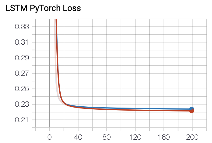
This is the loss graph. It is plotted cleanly. Red represents train, and blue represents val. The loss decreases more reliably than the LSTM implemented with numpy. It is better to use a framework.
Summary
In this article, we implemented RNN and LSTM with numpy to understand them and conducted light experiments. We also implemented LSTM using PyTorch.
References
https://masamunetogetoge.com/gradient-vanish https://qiita.com/naoaki0802/items/7a11cded96f3a6165d01 http://kento1109.hatenablog.com/entry/2019/07/06/182247 https://qiita.com/KojiOhki/items/89cd7b69a8a6239d67ca https://qiita.com/t_Signull/items/21b82be280b46f467d1b https://qiita.com/tanuk1647/items/276d2be36f5abb8ea52e