最急降下法
最急降下法を用いてを最小化してみる。
from typing import TypeVar
import numpy as np
from japanize_matplotlib import japanize
import matplotlib.pyplot as plt
from matplotlib.figure import Figure

japanize()

Number = TypeVar("Number", np.ndarray, float)


# 最小化する関数 f(x) = x^2
def f(x: Number) -> Number:
    return x**2


# f(x) の勾配 (導関数) df/dx = 2x
def gradient(x: Number) -> Number:
    return 2 * x
プロット関数の定義
def plot_steps(current_x: float, history_x: list[float], current_step: int) -> Figure:
"""
f(x)と最急降下法の軌跡をプロットする。
Args:
current_x: 最急降下法の現在のxの位置。
history_x: これまでのxの履歴のリスト。
current_step: 現在のステップ数。
Returns:
Figure: プロットの図オブジェクト。
"""
# f(x)のプロット用のデータを作成
x_curve = np.linspace(-5, 5, 100)
y_curve = f(x_curve)
# これまでに計算した点のデータを作成
history_y = f(np.array(history_x))
# プロットの作成
fig, ax = plt.subplots(figsize=(10, 6))
ax.plot(x_curve, y_curve, "b-", label="f(x) = x^2")
ax.plot(history_x, history_y, "ro--", label="最急降下法の軌跡", markersize=8)
ax.plot(current_x, f(current_x), "g*", markersize=15, label="現在の位置")
# ラベルとタイトルの追加
ax.set_title(f"最��急降下法: Step {current_step}")
ax.set_xlabel("x")
ax.set_ylabel("f(x)")
ax.legend()
ax.grid(True)
return fig
パラメーター設定
- 学習率:
learning_rate = 0.1 - 初期値:
initial_x = 4.0 - ステップ数:
total_steps = 3
学習率はxの更新をどれだけ大きく行うかを決定します。
learning_rate = 0.1
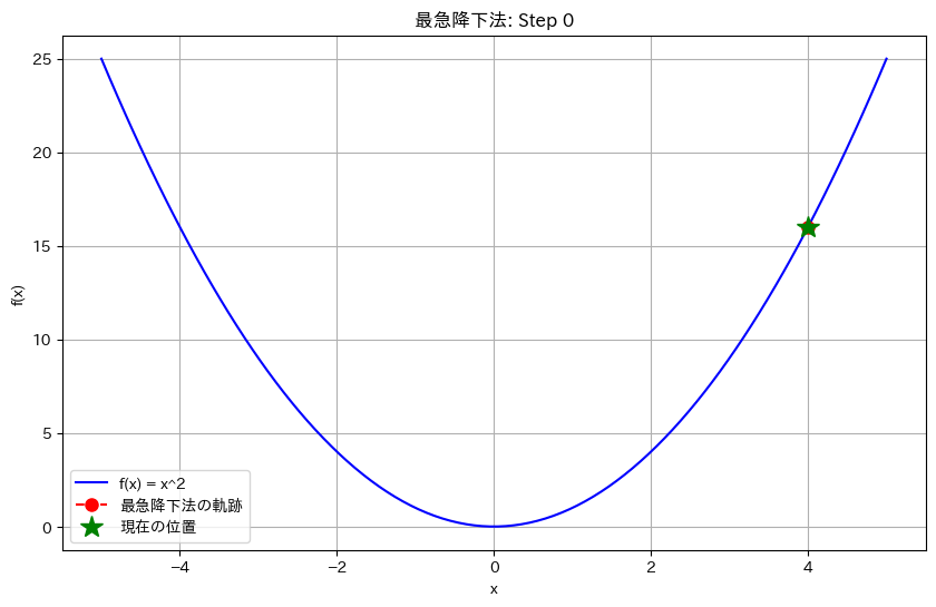
history_x = [current_x := 4.0]
total_steps = 3
plt.show(plot_steps(current_x, history_x, 0))
最急降下法を実行する
for i in range(total_steps):
    grad = gradient(current_x)

    # 最急降下法の更新ステップ
    # x_new = x_old - learning_rate * grad
    prev_x = current_x
    current_x = current_x - learning_rate * grad

    history_x.append(current_x)

    step_num = i + 1
    print(f"\nStep {step_num}:")
    print(f"  現在の位置: x = {prev_x:.4f}")
    print(f"  傾き ≈ {grad:.4f}")
    print(f"  新しい位置: x = {current_x:.4f}")
    print(f"  現在の関数値: f(x) = {f(current_x):.4f}")

    fig = plot_steps(current_x, history_x, step_num)
    plt.show(fig)
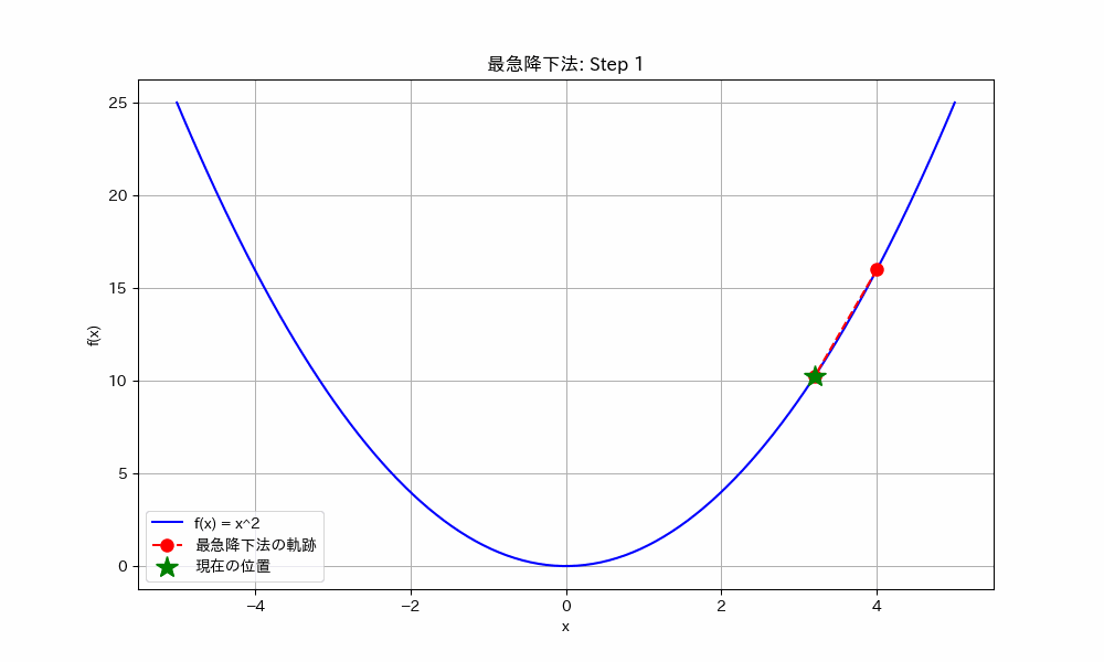
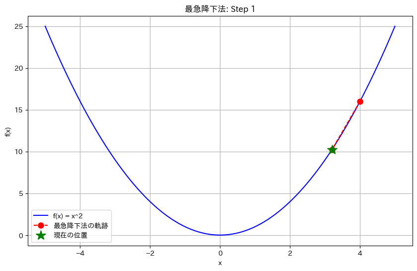
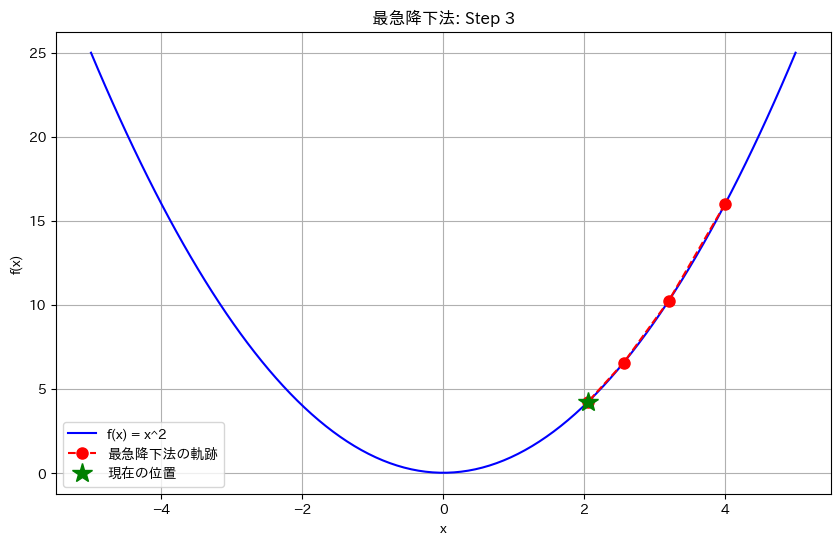
Step 1: 現在の位置: x = 4.0000 傾き ≈ 8.0000 新しい位置: x = 3.2000 現在の関数値: f(x) = 10.2400
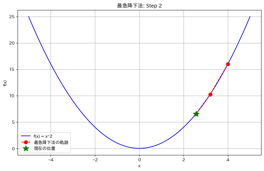
Step 2: 現在の位置: x = 3.2000 傾き ≈ 6.4000 新しい位置: x = 2.5600 現在の関数値: f(x) = 6.5536
Step 3: 現在の位置: x = 2.5600 傾き ≈ 5.1200 新しい位置: x = 2.0480 現在の関数値: f(x) = 4.1943
おまけ: より長いステップ数での最急降下法の様子
steps = 15
history_x = [current_x := 4.0]
history_figs = []

for i in range(steps):
    grad = gradient(current_x)
    current_x = current_x - learning_rate * grad
    history_x.append(current_x)
    history_figs.append(plot_steps(current_x, history_x, i + 1))

import imageio  # noqa

with imageio.get_writer(
    "gradient_descent.gif", mode="I", duration=0.5, loop=0
) as writer:
    for fig in history_figs:
        fig.savefig("temp.png")
        image = imageio.v2.imread("temp.png")
        writer.append_data(image)
        plt.close(fig)