A Summary of Summaries on Representation Learning

This is a summary of representation learning. Representation learning is a highly versatile learning approach that includes the recently popular self-supervised learning, and it holds potential for addressing a wide variety of tasks. It might be worth studying!

1. Representation Learning

The goal is to transform high-dimensional data such as images into lower-dimensional representations (embed them in a lower-dimensional space). The key is to lose as little information as possible while ensuring that each compressed representation carries some high-level meaning. The objectives include:

1. Reducing processing costs by converting to lower-dimensional representations
2. Abstracting and extracting more essential information to facilitate other downstream tasks
3. Improving adaptability to transfer learning through the above properties

1-1. Classification of Representation Learning

• Learning through tasks that improve accuracy
• Metric learning
• Deep generative models

1-2. Feature Extraction Without Learning

While research on information obtained from representation learning has been advancing, it remains difficult to clarify what each representation means. Depending on the desired features in an image, non-learning-based methods may suffice. A survey paper summarizing recent trends in this area is:

• Recent Advances in Features Extraction and Description Algorithms: A Comprehensive Survey. Ehab Salahat, Member, IEEE, and Murad Qasaimeh, Member, IEEE

2. Tasks That Improve Accuracy

2-1. Classification

• Supervised

  • "Full"-supervised
  • Semi-supervised
  • Weakly-supervised

• UnSupervised

  • Self-Supervised

2-2. Supervised

Here we list commonly used methods for extracting features from any layer of a neural network through some form of labeled learning, without distinguishing between conventional supervised learning (where all labels are available) and other approaches such as semi-supervised or weakly-supervised learning.

Classification

1. Semantic Segmentation
2. Object Detection
3. Image Captioning
4. Action Recognition

2-2-0. Summary

There is a truly diverse range of supervised methods for obtaining features. Currently, whether a neural network captures features is judged by the accuracy against the ground truth for the given task, but in reality, what features the network focuses on during learning has not been fully clarified.

From the perspective of feature extraction, it is not straightforward to determine what features each layer (and each channel within that layer) focuses on. Moreover, as demonstrated by adversarial machine learning, there is a view that networks do not actually capture features at a high semantic level. Personally, I felt that at the current stage, obtaining feature representations from intermediate layers of a neural network through accuracy-improving tasks is still challenging.

---

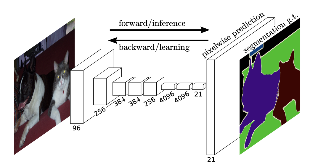
2-2-1. Semantic Segmentation

• Fully Convolutional Networks for Semantic Segmentation[Jonathan Long, Evan Shelhamer, Trevor Darrell]

---

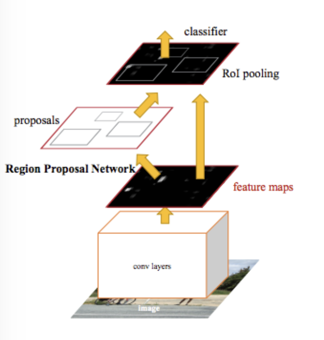
2-2-2. Object Detection

Object detection consists of a detection component that extracts regions likely to contain objects, and a recognition component that determines whether objects actually exist in those regions. Depending on the structure of the detection component, methods have been classified and improved as follows:

• Faster R-CNN Towards Real-Time Object Detection with Region Proposal Networks Separating the detection and recognition parts means that each detected region must be fed into the ConvNet individually, which incurs significant overhead. By first passing the image through conv layers and then detecting proposals from there, the overhead is reduced. In other words, detection and recognition can be completed within a single neural network and optimized jointly.

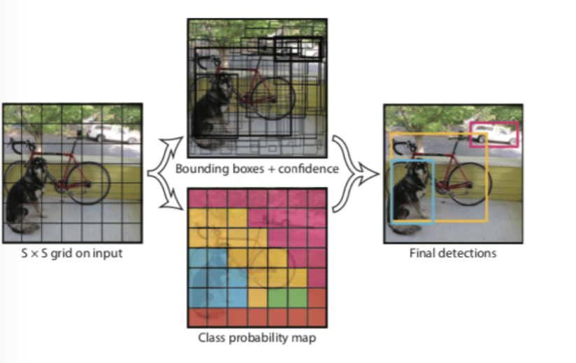
• YOLO: You Only Look Once: Unified, Real-Time Object Detection In Faster R-CNN, the recognition part processes the output of the detection part, meaning the processing pipeline is sequential and cannot be parallelized, causing latency. YOLO improves on this by enabling parallel processing.

---

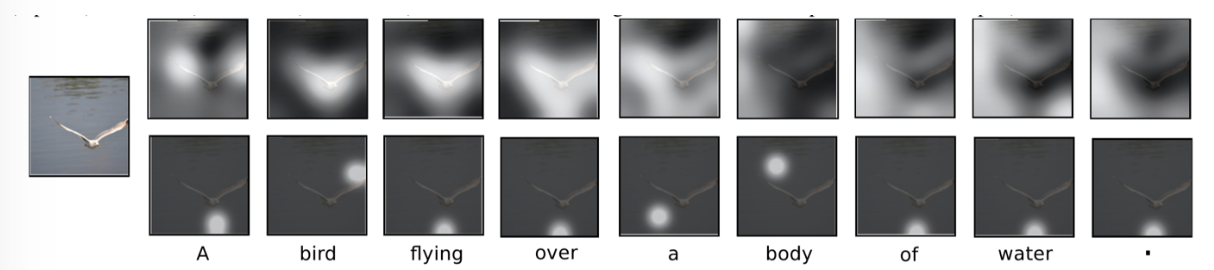
2-2-3. Image Captioning

Honestly, there are quite a variety of methods in this area and I was unable to get a complete overview. Below I provide a well-organized resource and a link to a survey paper.

• Show, Attend and Tell: Neural Image Caption Generation with Visual Attention

---

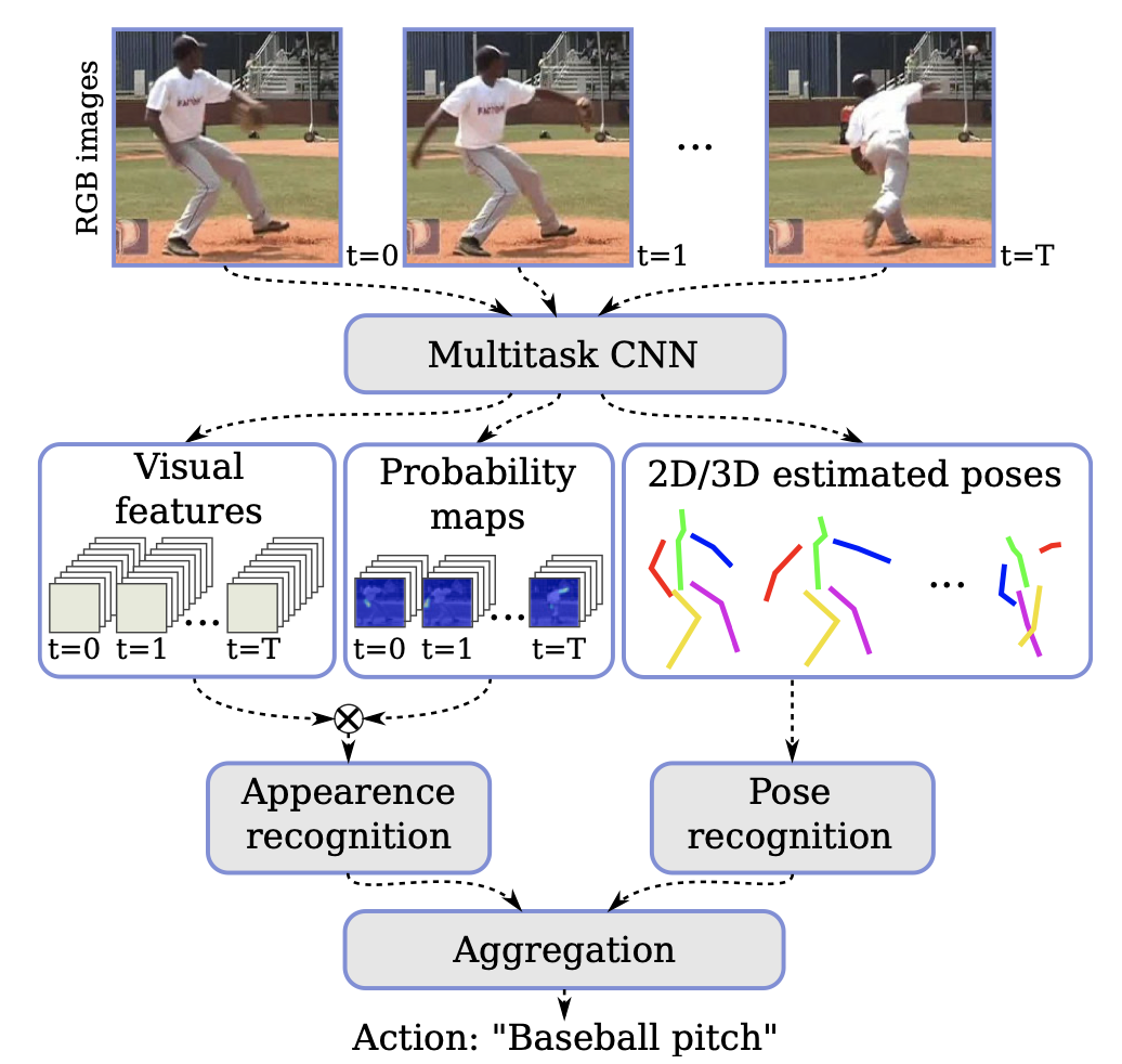
2-2-4. Action Recognition

You may also find results by searching for "Action Estimation." While some work addresses single still images, that overlaps with image captioning. The methods introduced below estimate what actions are being performed in continuous input data such as video.

• 2D/3D Pose Estimation and Action Recognition using Multitask Deep Learning [Diogo C. Luvizon, David Picard, Hedi Tabia]

2-3. Unsupervised

The following is written assuming the use of ConvNets. Although titled "Unsupervised," this section deals with self-supervised learning. While generative models such as GANs could be considered unsupervised, they are treated separately.

Brief Explanation

Self-supervised learning uses input data without labels. Self-supervised methods perform pretext tasks to obtain feature representations of the data that are useful for the desired target tasks. Various approaches for these pretext tasks have been proposed, which are briefly summarized below.

Additionally, using values learned through self-supervised methods as initial weights for a neural network can prevent overfitting and improve classifier accuracy.

Pros and Cons

• Pros
  • No need to prepare labeled data
  • Easier to understand (and easier to make complex architectures) compared to generative models
• Cons
  • Difficult to evaluate whether the obtained representations are actually good on their own
  • Currently, evaluation requires running the target task, which ultimately requires ground truth

Specific Methods

Specific methods can be broadly categorized into the following four types: 1. Context-Based 2. Free Semantic Label-Based 3. Cross Modal-Based 4. Generation-Based

2-3-0. Summary

According to the referenced papers, the method that best captured features from still images was DeepClustering. It achieved accuracy close to supervised methods across all tasks: classification, detection, and semantic segmentation. On the other hand, for video, CubicPuzzle achieved the highest accuracy, but there was still a significant gap compared to supervised methods.

From the perspective of representation learning, it remains unclear what features each self-supervised method focuses on, just as with supervised methods. Furthermore, whether self-supervised methods actually focus on good features is evaluated by performing supervised tasks using a network with transferred parameters, making it impossible to confirm on its own whether the features are truly good.

---

2-3-1. Context-Based

Methods that attempt to understand the content of images and videos. The advantage is that they are easy to implement and understand conceptually. They also have high compatibility with various tasks. The drawback is that it is unclear whether the pretext tasks are being performed based on high-level semantic understanding. For example, even in a puzzle rearrangement task, the model might only be looking at colors or edge connections to solve it.

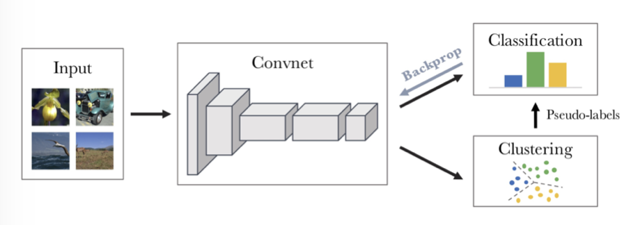
• DeepCluster Deep Clustering for Unsupervised Learning of Visual Features [Mathilde Caron+, ECCV2018] First, input images are fed into a ConvNet to obtain feature maps. Only the ConvNet is used for feature maps; fully connected layers are not used at this stage. PCA and L2 normalization are applied to the feature maps for dimensionality reduction, then k-means is performed to assign pseudo-labels. Training is conducted as classification based on these pseudo-labels.

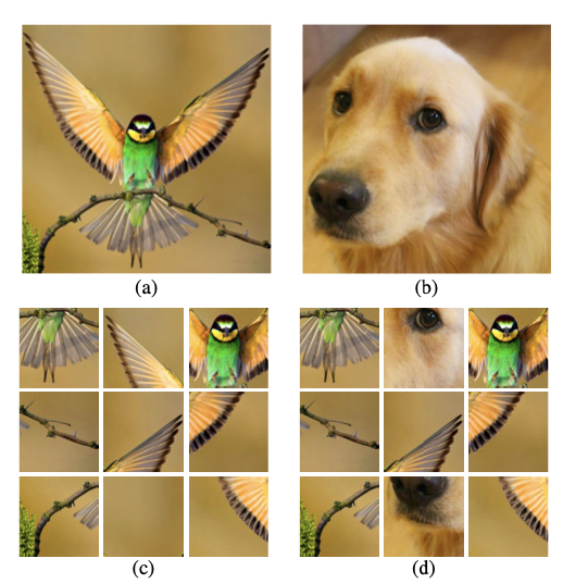
• Jigsaw Puzzle++ Noroozi et al., "Boosting Self-Supervised Learning via Knowledge Transfer", CVPR 2018. Solve puzzles created by combining two images.

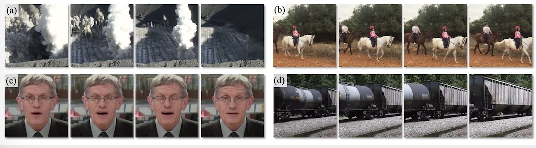
• Learning and Using the Arrow of Time Donglai Wei, Joseph Lim, Andrew Zisserman and William T. Freeman Harvard University University of Southern California University of Oxford Massachusetts Institute of Technology Google Research Determine whether time is progressing forward or backward in a video.

---

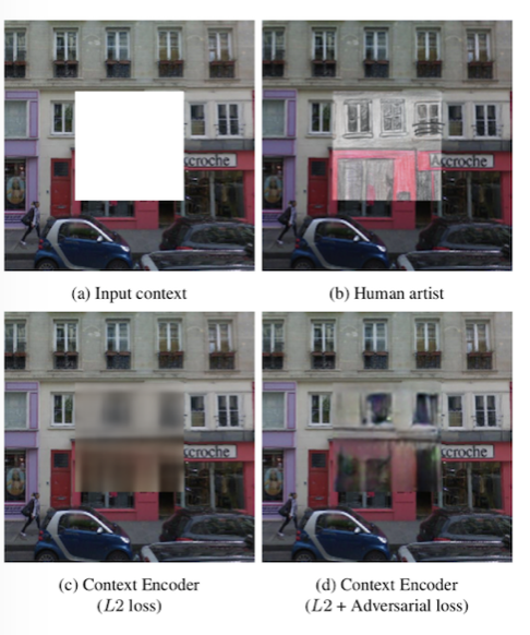
2-3-2. Generation-Based

The referenced paper included VAEs and GANs under Generation-Based, but here they are treated separately as generative models. Generation-Based here refers to methods that use a neural network to reconstruct input data from which some information has been removed.

• Context Encoders: Feature Learning by Inpainting Have a neural network reconstruct an image from which a portion has been cropped out.

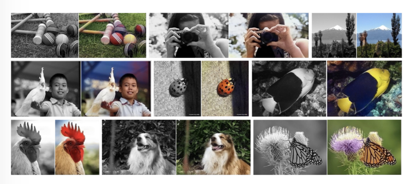
• Colorful Image Colorization Have a neural network colorize input images from which color information has been removed.

---

2-3-3. Free Semantic Label-Based

Methods that use label data created without human interpretation for training. (Calling this unsupervised learning feels a bit like cheating.) Labels without human interpretation include depth, segmentation masks, surface normal information, etc. This information is typically obtained through rendering in games and similar environments. The advantage is that it is easier to make the model capture features compared to other self-supervised methods. The drawbacks include the need to create hardware capable of such rendering, and the fact that labels generated by hardware rendering tend to be noisy.

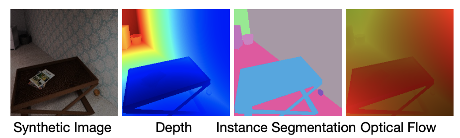
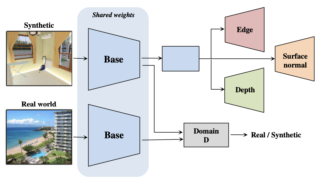
• Cross-Domain Self-supervised Multi-task Feature Learning using Synthetic Imagery[Zhongzheng Ren and Yong Jae Lee University of California, Davis] Train on synthetic images generated by hardware rendering, then perform domain adaptation on real-world images.

---

2-3-4. Cross Modal-based Learning

An approach that leverages continuity in video input data as constraints for learning. Specifically, data that is continuous in video includes RGB values, optical flow, audio data, and camera pose.

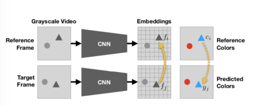
• Tracking Emerges by Colorizing Videos[Carl Vondrick, Abhinav Shrivastava, Alireza Fathi, Sergio Guadarrama, Kevin Murphy] Based on the premise that an object moves across consecutive frames but its color remains the same, the model can learn object motion without human-provided labels.

3. Metric Learning

3-1. Classification

• Metric Learning
  • Contrastive Learning
  • Others

3-2. Contrastive Learning

Here, contrastive learning is defined as methods that involve concepts such as "positive pairs" and "negative pairs" in the context of metric learning.

Some say that contrastive learning is a term used in the context of self-supervised learning, and that those working on metric learning in a broader sense do not use the term "contrastive learning," but I could not find a strict definition.

Classification

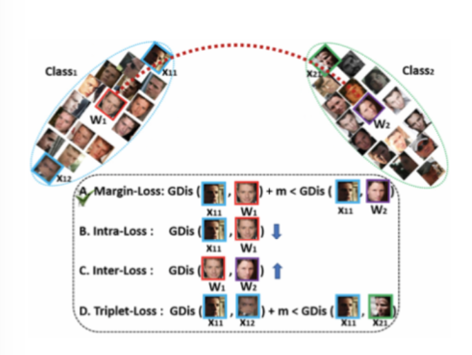
• Contrastive loss
• Triplet loss + $\alpha$

3-2-1. Contrastive loss

Deep metric learning started with the invention of contrastive loss, and the network incorporating contrastive loss was the siamese network. However, contrastive loss itself is no longer widely used; instead, triplet loss and its variants (shown below) are used. Contrastive loss has also evolved beyond simply feeding two images and pushing their embedding distances apart, incorporating various improvements.

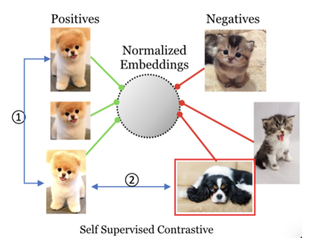
• SimCLR A Simple Framework for Contrastive Learning of Visual Representations Rather than simply feeding images as input, data-augmented images are used. The contrastive loss is also improved to become what can be called a self-supervised contrastive loss, expressed in terms of distances in an embedding space represented on a unit hypersphere.

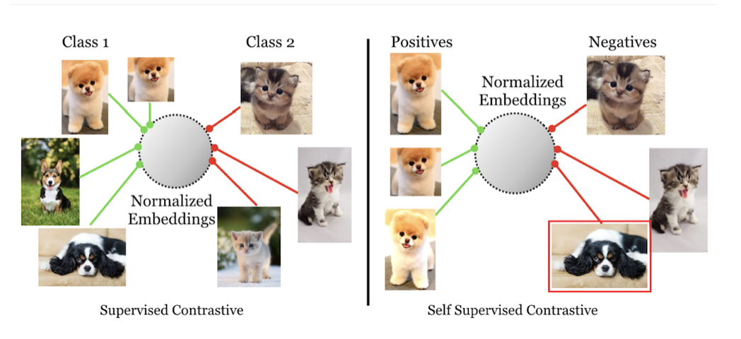
• Supervised SimCLR Supervised Contrastive Learning An improvement on SimCLR. Since standard SimCLR is self-supervised, its embedding space representations do not consider whether samples originally belong to the same class. However, intuitively, images of the same dog should be closer together than images of a cat. This paper incorporates that intuition.

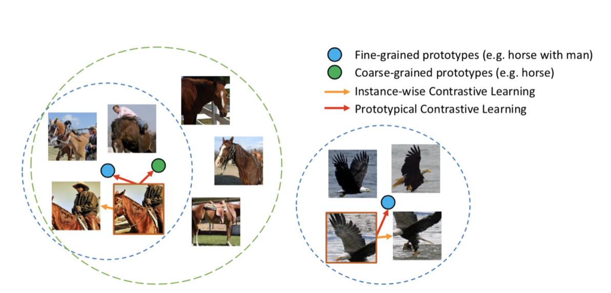
• Prototypical Contrastive Learning Prototypical Contrastive Learning of Unsupervised Representations This shares the same philosophy as Supervised SimCLR but is a completely unsupervised approach. The underlying idea is that images that are similar as inputs should also be similar in the embedding space. By first clustering input images with k-means into prototypes and then performing metric learning based on these prototypes, accuracy was improved.

  Horse images are not only closer to other horse images than to bird images, but within the group of horse-related images, images of people riding horses are properly distinguished from images of horses alone.

3-2-2. Triplet loss + $\alpha$

Methods that emerged to address the problems of contrastive loss, which was used at the beginning of deep metric learning. However, these introduced new problems that were not present before, requiring further improvements. For details, please refer to this article.

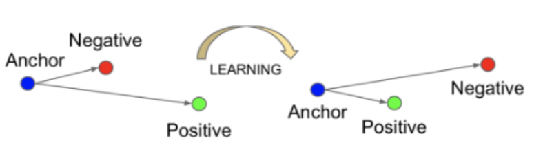
• FaceNet A Unified Embedding for Face Recognition and Clustering The most basic method using triplet loss.

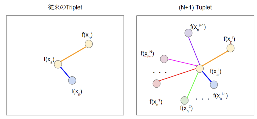
• N+1 Tuplet Improved Deep Metric Learning with Multi-class N-pair Loss Objective A method that generalizes triplets to N. Since it compares against more points, the behavior should be more stable.

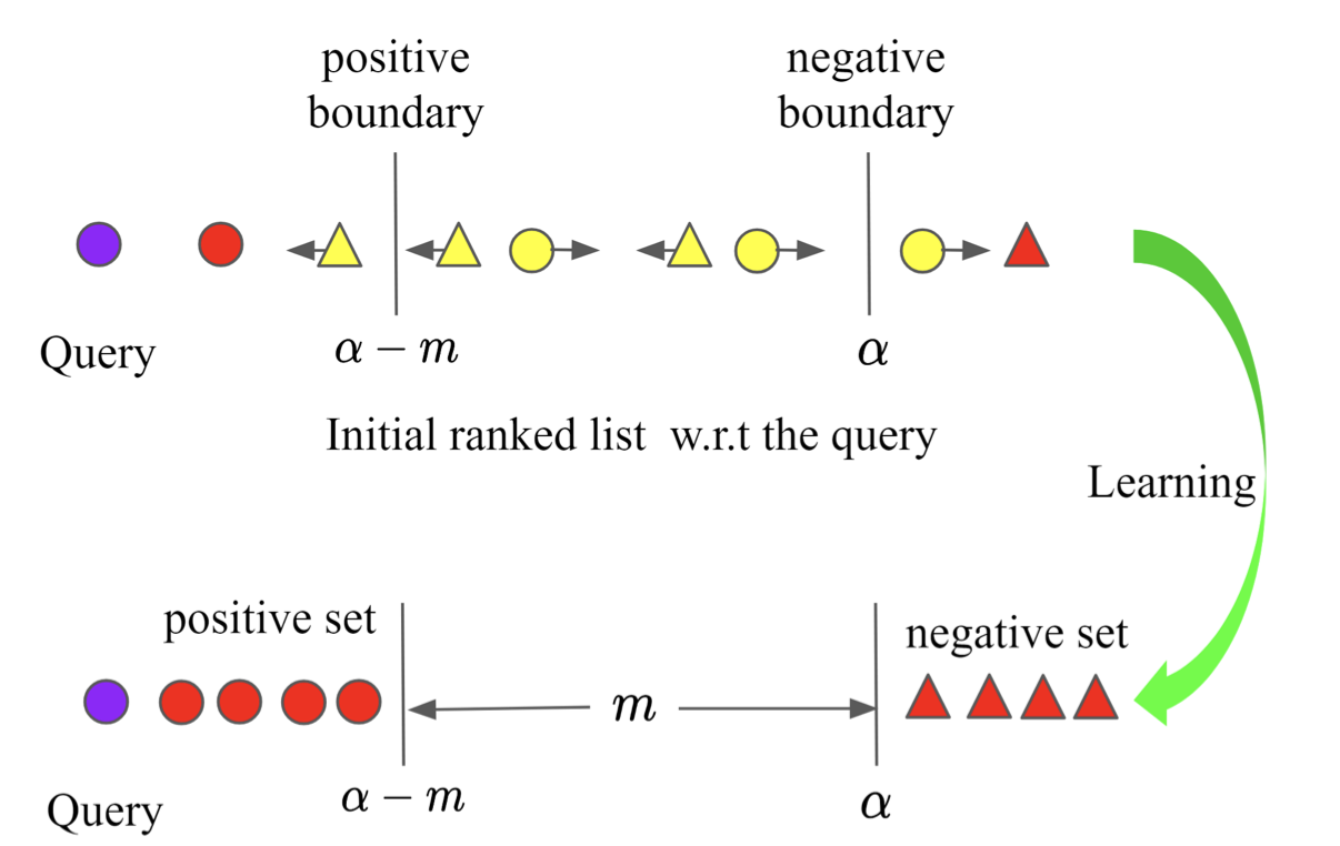
• Ranked List Loss Ranked List Loss for Deep Metric Learning Instead of selecting specific samples, all samples are considered, ensuring that no effective training pairs are missed. Additionally, while conventional methods would keep pushing positive pairs closer indefinitely, this method establishes a threshold beyond which pairs need not be made closer. (This method might be better categorized as an evolution of contrastive loss.)

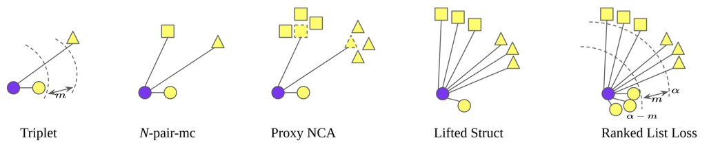
Comparison with methods up to Ranked List Loss.

3-3. Others

Methods in metric learning that do not involve the terms "positive pair" or "negative pair" are grouped here. That is, methods that do not use contrastive loss or triplet loss for training. This might reflect insufficient research on my part, but it seems that most metric learning approaches are discussed in the context of contrastive learning...

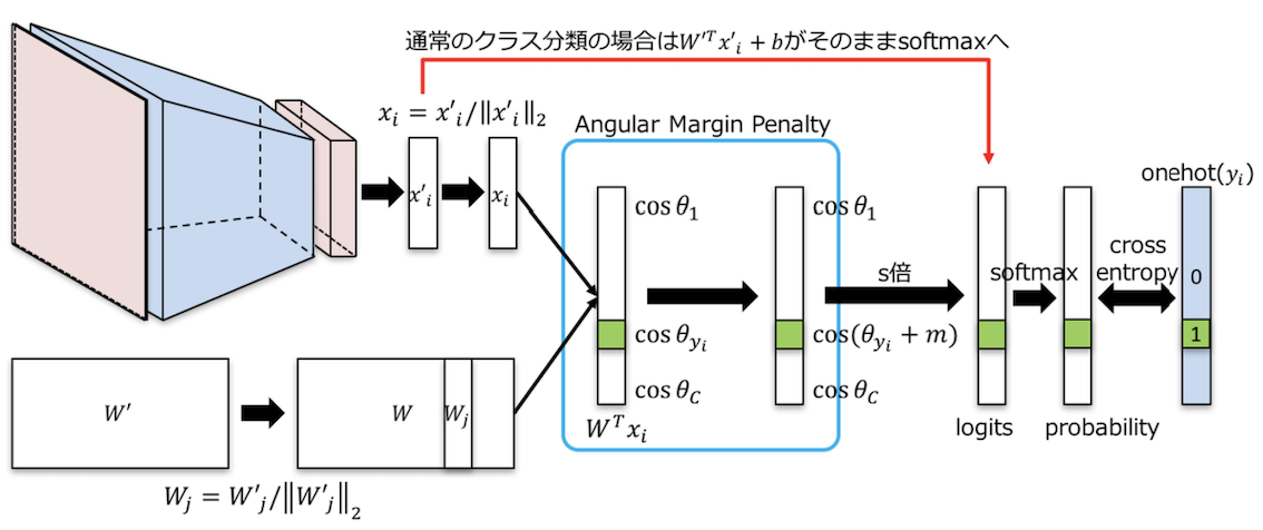
3-3-1. ArcFace

Additive Angular Margin Loss for Deep Face Recognition By representing the embedding space as a hypersphere, the position of each latent variable can be expressed as an angle in the embedding space. The angle between each class and the representative W is expressed as $\cos\theta$. The parameter $\theta$ is updated so that different classes become further apart.

4. Deep Generative Models

Generative models are a type of unsupervised model. Here, generative models are treated separately from the semi-supervised model framework discussed above. The reason is that the latent variables obtained by the encoder of a generative model are highly abstracted data, and the latent space can be designed to have disentangled relationships.

4-1. Classification

• VAE
• GAN

4-2. Disentangled Representations and Distributed Representations

When reducing the dimensionality of input data and transforming it into representations with higher-level meaning, the resulting representations have fewer dimensions than the input. The new representations are formed by distributing and combining components of the input data, which is called a distributed representation. In a distributed representation, each individual representation does not necessarily independently affect the output.

On the other hand, when each of these new representations has an independent relationship with the output, they are called disentangled representations. Ideally, changing a single latent variable should cause only one feature to change in the output. With disentangled representations, it becomes easier to understand what each latent variable controls in the output. Representations where we can understand what feature each variable relates to are called interpretable representations.

4-3. Evaluation of Disentanglement and Decomposition

Currently, there is no absolute evaluation method for disentanglement, and new evaluation methods are proposed alongside each new disentangled representation learning approach, resulting in a proliferation of evaluation metrics.

Considering what disentanglement should ideally look like, it can be thought of as consisting of two main components: 1. The disentangled latent variables are linked to understandable features and can be manipulated. 2. The structure of the latent space is correctly extracted and can be handled.

Point 1 means being able to understand what changes in the generated image when latent variable $z_i$ is varied, and current evaluation metrics focus on this aspect. Personally, I think this aspect of point 1 can also be called interpretable.

On the other hand, point 2 means that information composed of multiple elements (such as ethnicity) should also be composed of multiple elements in the latent space. Therefore, when we want to handle such multi-element information, we need to understand the structure of the latent space. Current evaluation metrics do not adequately address this aspect.

The term decomposition has been proposed as a concept encompassing point 2 as well.

4-4. Pros and Cons of Deep Generative Models

• Pros
  • No need to prepare labeled training data (except for supervised GANs)
  • If disentangled representations can be obtained, they may be transferable to other tasks
• Cons
  • Difficult to increase representation capacity by making the network deeper

4-5. VAE

Classification

• Adding regularization terms
• Methods using hierarchical latent representations extracted at different depths

Brief Explanation

The objective function of VAE is expressed as follows:

$$\log p(x)=D_{KL}[q(z|x)||p(z|x)] + L(x,z)$$

Here, $L(x,z)$ is the evidence lower bound (ELBO), which is derived as:

$$L(x,z) := \underbrace{\mathbb{E}_{q(z|X)}[\log p(x|z)]}_{\rm (i)} - \underbrace{D_{KL}[q(z|x)||p(z)]}_{\rm (ii)}$$

Maximizing this evidence lower bound means building a good model that represents the data distribution $p(x)$. The evidence lower bound consists of two components ${\rm (i), (ii)}$.

The goal is to maximize each of these: 1. $\mathbb{E}\_{q(z|X)}[\log p(x|z)]$: Reconstruction error This first term can be thought of as representing the accuracy of the autoencoder itself, indicating how close the output $X'$ is to the input data $X$ after passing through the encoder and decoder.

2. $-D_{KL}[q(z|x)||p(z)]$: KLD term This is the KL divergence term expressing how close the probability distributions $q(z|x)$ and $P(z)$ are. The closer the two distributions, the larger this $-D_{KL}[q(z|x)||p(z)]$ term becomes overall (note the minus sign). In VAE, $p(z)$ is assumed to be a standard normal distribution, meaning it evaluates how close the latent space to which input data $X$ is mapped is to a standard normal distribution.

4-5-1. Adding Regularization Terms

From the perspective of wanting disentangled representations, when considering how to design a VAE, we consider the approximate posterior $q(z|x)$ in the second term to be close to a standard normal distribution as having disentangled representations. The following methods of adding regularization have been proposed:

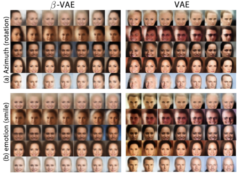
• Beta-VAE LEARNING BASIC VISUAL CONCEPTS WITH A CONSTRAINED VARIATIONAL FRAMEWORK[Irina Higgins, et al.] A regularization term $\beta$ is added to the second term of the evidence lower bound, resulting in the following. This design ensures that $L(x,z)$ cannot become large unless the approximate posterior is closer to a standard normal distribution than in "Vanilla" VAE. While "Vanilla" VAE changes other elements such as facial features and hair when trying to change a single element (angle or degree of smile), $\beta$-VAE reduces the impact on other elements.

  $$L(x,z) := \mathbb{E}_{q(z|X)}[\log p(x|z)]-\beta\cdot D_{KL}[q(z|x)||p(z)]$$

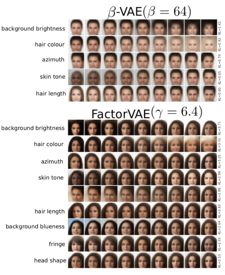
• FactorVAE Disentangling by Factorising [Hyunjik Kim, Andriy Mnih] Over-emphasizing the second term caused the reconstruction error to be neglected, resulting in blurry generated images. Focusing on the second term of $\beta$-VAE, it can be further decomposed as:

$$-\beta \cdot D_{KL}[q(z|x)||p(z)] = -\beta \cdot \bigl\{ \underbrace{-I(x;z)}_{\rm (i)} + \underbrace{L_{KL}(q(z),p(z))}_{\rm (ii)}\bigr\}$$

$\rm (i)$: Dependency between input $X$ and latent variable $z$, $\rm (ii)$: Discrepancy between the marginal distribution of z and the prior distribution. From this, minimizing the second term in $\beta$-VAE to maximize the evidence lower bound was reducing the mutual information in $\rm (i)$, increasing reconstruction error. To correct this, a correction term was incorporated into the objective function. Specifically, a Total Correlation constraint was added. As shown below, more features can be extracted independently compared to $\beta$-VAE. However, some argue that it does not work well on non-face data. (Are facial features easier to classify?)

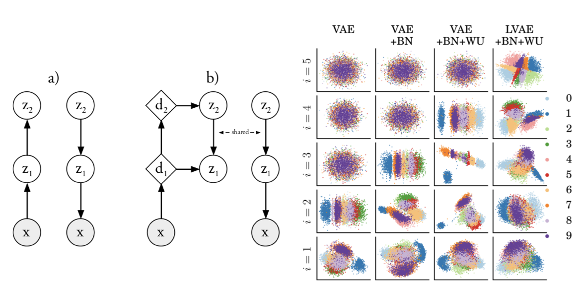
4-5-2. Methods Using Hierarchical Latent Representations Extracted at Different Depths

• LVAE Ladder Variational Autoencoders(Casper Kaae Sonderby, Tapani Raiko, Lars Maaloe, Soren Kaae Sonderby, Ole Winther)

While conventional VAEs obtain latent variables only from the final layer, LVAE obtains latent variables with different levels of abstraction from each depth. In VAEs, when obtaining latent variables only from the final layer, adjusting those variables is difficult when there are many layers in between. By obtaining variables from each layer, representation capacity is improved. Additionally, this paper uses a regularization term $\beta$ similar to $\beta$-VAE, and demonstrates that performance improves by gradually increasing $\beta$ from 0 to 1 according to training progress (Warm-Up).

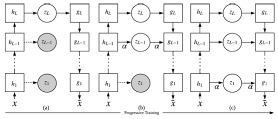
• pro-VAE Progressive Learning and Disentanglement of Hierarchical Representations[Zhiyuan Li, Jaideep Vitthal Murkute, Prashnna Kumar Gyawali, Linwei Wang] pro-VAE introduces Progressive Learning to the above LVAE. Initially, only the deepest and most abstract latent variables are extracted, and as training progresses, features from shallower layers are gradually incorporated as latent variables.

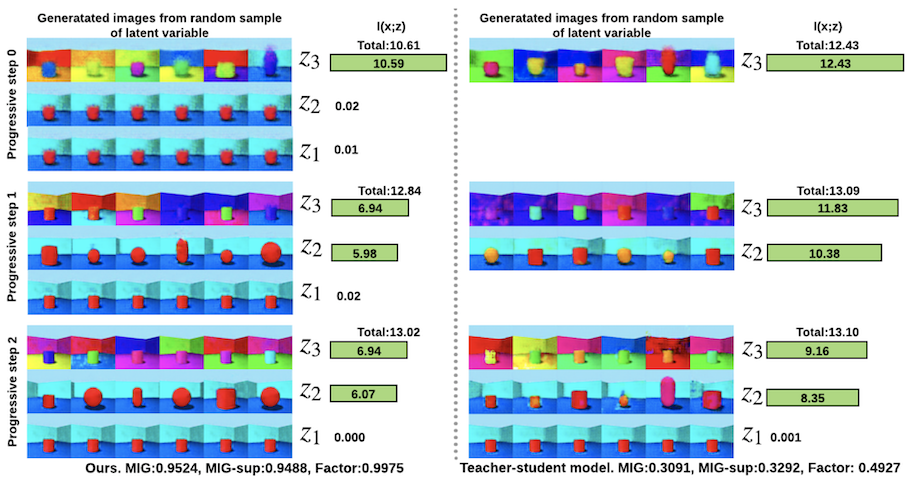
The figure below compares the performance of pro-VAE with a teacher-student model that can be thought of as pro-VAE without the ladder component. Comparing the changes in generated images when varying latent variables from each layer of pro-VAE versus changes from the final layer of the teacher-student model shows that pro-VAE successfully extracts more disentangled latent variables as training progresses and more layers are used for generation.

4-6. GAN

Representation learning to obtain disentangled representations through GANs is categorized and introduced as follows. The attempt to obtain disentangled representations through GANs began with InfoGAN. InfoGAN itself has unstable training and is no longer used, but it pioneered disentangled representation learning.

InfoGAN Interpretable Representation Learning by Information Maximizing Generative Adversarial Nets [Xi Chen, Yan Duan, Rein Houthooft, John Schulman, Ilya Sutskever, Pieter Abbeel]

Classification

The reason some GANs are supervised is that classifiers trained on the dataset are needed to judge whether changes in the latent space are disentangled.

• Supervised
• Self-supervised
• Unsupervised

4-6-0. Summary

Since disentangled representation learning with GANs is a recently emerging research field, all methods are new and not extensively studied yet, making it impossible to definitively say which is best. Based on the current papers, my impressions are as follows. However, each paper claims its own research is superior...

• Supervised Cost: Poor, Representation: Fair
• Self-supervised Cost: Fair, Representation: Fair
• Unsupervised Cost: Good, Representation: Good

4-6-1. Supervised GAN

• StyleGAN Interpreting the Latent Space of GANs for Semantic Face Editing[Yujun Shen, et al] A classifier must be trained in advance for each assumed latent variable. So the expected features of the latent space are predetermined before training. If so, this might be convenient in its own way. However, reproducibility would likely be low without very careful design.

4-6-2. Self-supervised GAN

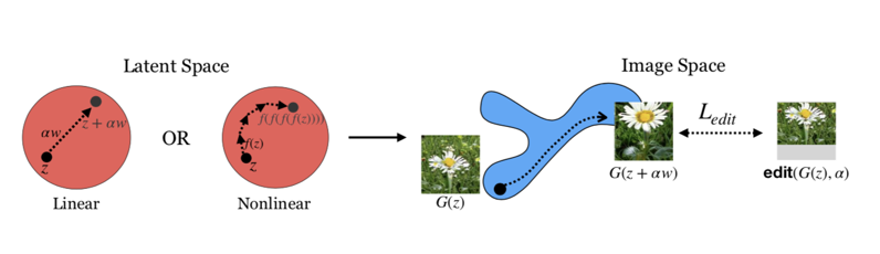
• ON THE "STEERABILITY" OF GENERATIVE ADVERSARIAL NETWORKS[Ali Jahanian, Lucy Chai, Phillip Isola] Disentangled representations in the latent space for features that can be obtained through simple image editing (such as zoom and color tone) can be acquired through self-supervised methods. Also, how far each latent variable can be varied depends on the variance of the input data.

4-6-3. Unsupervised GAN

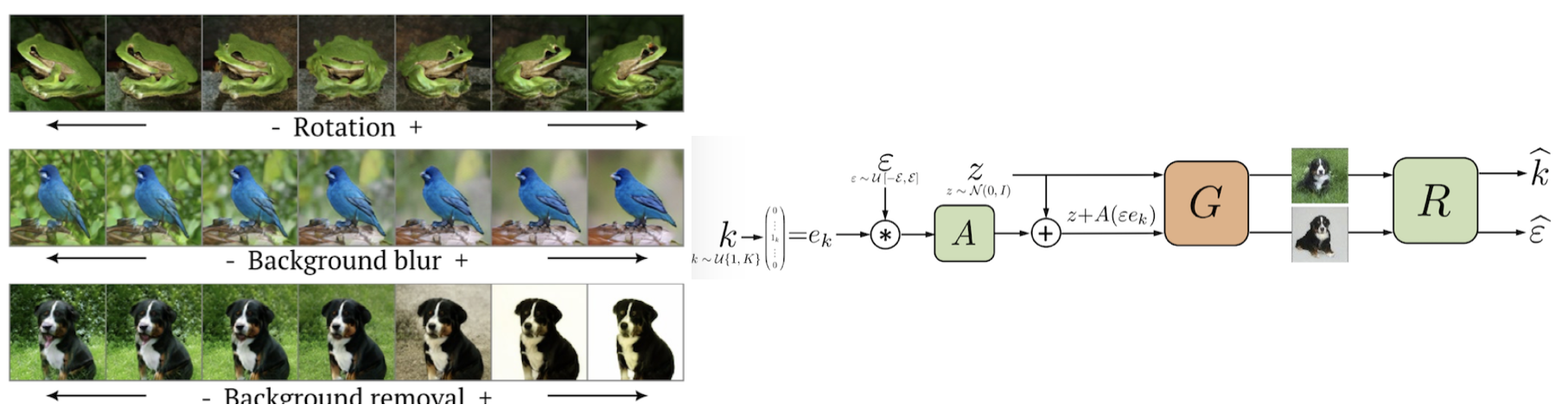
• Unsupervised Discovery of Interpretable Directions in the GAN Latent Space [Andrey Voynov Artem Babenko] In addition to capturing features such as rotation similar to other supervised methods, this method also captures background regions. The authors claim this demonstrates greater representation power than other GAN-based methods. They also presented examples where background detection could be applied to weakly-supervised semantic segmentation and similar tasks.

References

Websites

• Personally Interesting Machine Learning Papers in 2019
• Deep Learning: A Survey of Surveys
• Self-Supervised Representation Learning
• Feature Representation Learning with Self-supervised Learning
• New Method for Disentangled Representation Learning: Progressive VLAE Explained!
• Verification of Unsupervised Disentangled Representation Learning Methods
• Deep Learning from the Perspective of Mutual Information
• Awesome Image Captioning
• Disentanglement Survey: Can You Explain How Much Are Generative Models Disentangled?
• Theory of Variational Inference
• Introduction to Deep Generative Models for PRML Learners

Papers

• Recent Advances in Features Extraction and Description Algorithms: A Comprehensive Survey [ Ehab Salahat, Member, IEEE, and Murad Qasaimeh, Member, IEEE]
• Self-supervised Visual Feature Learning with Deep Neural Networks: A Survey [Longlong Jing and Yingli Tian⇤, Fellow, IEEE]
• A Comprehensive Survey of Deep Learning for Image Captioning